Project - De Compression Competition
Group X
Teppo Niinimäki, Pekka Parviainen
This document reports the work we have done at the Information-Theoretic Modelling Project. The project required a lots of effort. However, we enjoyd the project and it also teached us many new things (like how to write extremely short code).
The following table summarizes the progression of our compression system. As it can be seen we started working early and the progress after the first two weeks was small.
| Round | decomp. | curve1 | curve2 | info | letter | mushr. | rat | Bean1 | GroupX1 | Juusto1 | forest | GroupX2 | Juusto2 | Total |
|---|---|---|---|---|---|---|---|---|---|---|---|---|---|---|
| 1 | 1777 | 3108 | 6479 | 437 | 1697 | 1 | 3228 | 16727 | ||||||
| 2 | 1519 | 3108 | 6479 | 437 | 1329 | 64 | 3228 | 891 | 1 | 1729 | 18785 | |||
| 3 | 1606 | 3108 | 6478 | 437 | 706 | 64 | 3228 | 9388 | 1 | 1982 | 26998 | |||
| 4 | 1611 | 3108 | 6468 | 286 | 678 | 64 | 3187 | 9396 | 1 | 1982 | 26781 |
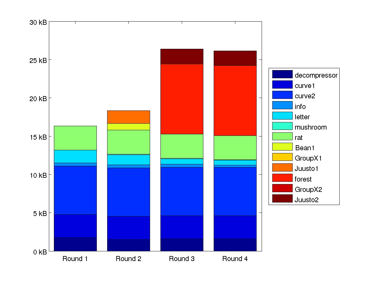
Letter was the only data set that saw some serious improvements. The pseudo improvement in info on the last round was primarily result from moving part of the data from compressed file to the decompressor. The progression and comparative sizes of compressed data sets are further illustrated by the figure 1.
Next we shall briefly describe how we ended up to these results.
Description of compression algorithms
curve1
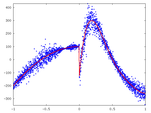
Coding of curve1 started with plotting the data on y-axis and sidedata on x-axis. The positive and negative x-values seemed to come from separate datasets and therefore we fitted a polynomials for the left side and right side separately. The degrees of these polynomial were 2 and 5, respectively. See figure 2.
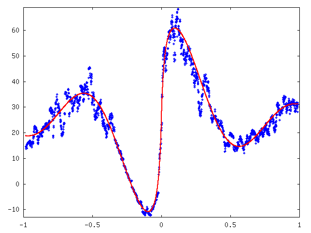
Next, we subtracted approximated mean curves from y-values and plotted standard deviation for each consecutive 30 values sequence with resulting values between -0.216 and -0.022 inversed. Then we fitted curve 25 + 50 sin(8x) / (|8x| + 0.2) by hand. See figure 3.
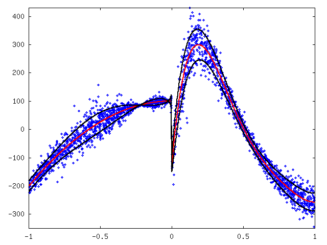
Figure 4 shows original values plotted with approximated mean and standard deviation.
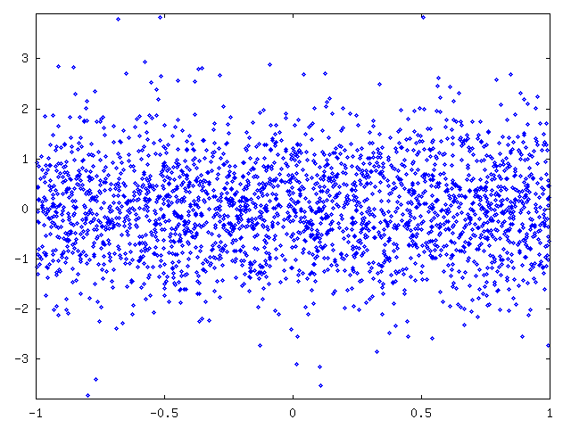
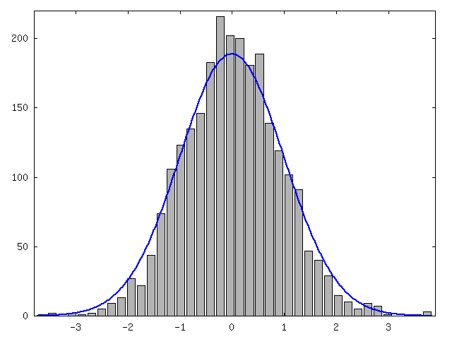
We further normalized the original values, that is, we subtracted mean and divided each value by standard deviation (figure 5). We plotted the distribution of normalized values and standard normal distribution (figure 6). As a conclusion we saw that normal distribution seemed to fit and we could use a normal distribution with mean and variance from the fitted function to compress data with arithmetic coding. We notice that values of curve1 are given in precision of 0.1. Now at any given x coordinate we can code the y coordinate as an interval of length 0.1 whose probability can be extracted from a normal distribution whose mean is given by the fitted polynomial and variance is given by the sin-curve.
curve2
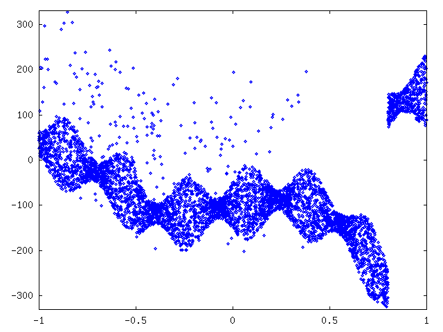
As with curve1 we started by plotting the data. See figure 7.
To make fitting a function we inversed and shifted values with x > 0.8 and shifted values with x < -0.5. Then, we fitted a 9-degree polynomial (red) and approximated maximum deviation by hand with some marginal added (black). See figure 8.
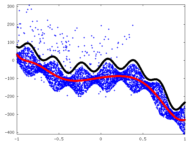
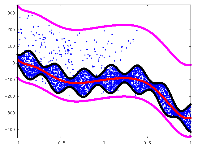
We removed outliers above the black line in the previous figure 8. After that we fitted mean curve (red) again. We then approximated maximum deviation again to be 55 + 30 sin(20x) (black) and approximated limits for outliers to be μ - 110 and μ + 320 (magenta) where μ is the approximated mean (red curve). Figure 9.
Now we were ready to compress data. We used arithmetic coding with data modeled using a weighted sum of two uniform distributions: one between black lines and another between magenta lines.
info
The info file consisted a header, a tricolor, and some text over the tricolor. Header was very hard to compress as opposed to the very compactly compressable tricolor. Our compression algorithm works in two phases such that first it writes the header and produces the tricolor. Then, it writes the text.
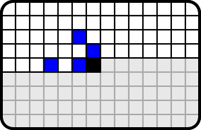
We coded text using conditional distributions and arithmetic coding. The figure 10 below shows the context of a pixel. The target pixel is black. When decoding that pixel we already know colours of pixel that are above it or at left on the same level (white). The blue squares define the pixel on which the target pixel's color is conditioned on. The choice of context seems to be somewhat unintuitive, but it is provided by an optimization algorithm.
letter
Letter was the dataset with the most progress over time. In the first round we used a nearest-neighbor search variant. For each of the items we sorted its predecessors based on the Euclidian distance to the given item. Then we counted how many different letters are found before we found a neighbor that is equivalent to the letter in question. The compressed file was achieved by coding these values arithmetically.
In the second round we improved our results by adding a preprocessing step, where items where ordered based on the sidedata before the nearest-neighbor search started.
In the third round, we developed a whole new strategy. For every item we computed weighted distance to all of its predecessors. Then we transformed these distances into value f = 1 / (s + dk) where d is the distance and s and k are parameter values. In next step we summed f-values for each letter to form unnormalized distribution. After distribution was normalized, we used arithmetic coding. Values for weights and parameter were chosen using a greedy optimization algorithm.
In the fourth round we used the same method as in the round three. However, this time we had better parameter values.
mushroom
Mushroom data set was the easiest to compress. The mushroom.info file contained description of a simple classifier with 100% accuracy. We implemented to a small Perl script which read side information and printed the correct symbol which allowed us to have a compressed file of size 1 byte.
During the second round we realized that combined size of the decompressor and the compressed file can be decreased by few bytes when the classifier is stored in the compressed file. Hence the size of the compressed file grew.
The aforementioned classifier classified mushrooms as poisonuos if the condition odor=NOT(almond.OR.anise.OR.none) OR spore-print-color=green OR (odor=none.AND.stalk-surface-below-ring=scaly.AND.(stalk-color-above-ring=NOT.brown)) OR (habitat=leaves.AND.cap-color=white) holds. Otherwise, mushrooms are edible.
rat
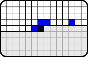
Compression of rat was done using conditional probability and arithmetic coding same way as the compression of the text in info dataset. The context can be seen in figure 11.
forest
Forest dataset was compressed using the same method as the letter dataset. However, two changes were made: Firstly we didn't perform initial sorting, and secondly we didn't use all preceeding values in encoding but a maximum of 718 previous values. The first choice was made because it notably increased compressibility. The second change was originally to keep (de)compression time reasonable low but it also seemed to work suprisingly well. Parameter values were chosen based on a greedy search algorithm.GroupX
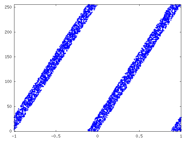
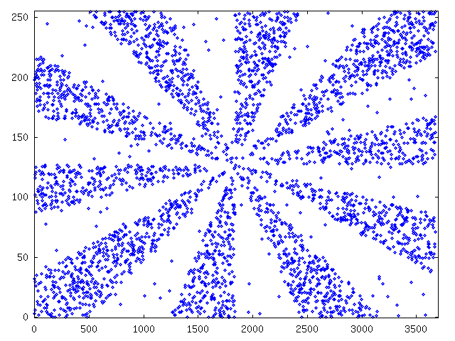
Our first dataset was constructed by first taking a number from curve2-sidedata, multiplying it by 256, adding a random number between 0 and 32 and taking modulo 256 over the number. Therefore, every byte could be compressed by 3 bits. The figure 12 shows values of curve2 sidedata on x-axis and values of GroupX-data on y-axis.
The second extra data set was constructed differently. For each byte we chose its value from a weighted mixture of uniform distribution. Distributions were chosen so that when plotted values formed the figure 13.
Other
Data provided by other groups seemed to be completely random and standard compression tools weren't able to compress these files. Therefore, we didn't compress these data sets.
Implementional Issues
In this section we explain some implementional solutions. We decided to use Octave as our primary programming language, because it provided many useful features that can be used to produce compact source code. In addition Perl was used to decompress mushroom data set as mentioned and shell scripts in compress.sh and decompress.sh did the selection of the right compressor and decompressor.
One of key factors to our success was to keep the decompressor compact. Therefore, decompressors for different data sets shared several scripts:
- adec.m, adec_opt.m, A.m
- Arithmetic decoding
- readbits.m, readbits_opt.m, B.m
- Reads the rest of the input and interpret as bits
- envdec.m, envdec_opt.m, E.m
- Loop for extracting data coded with context based arithmetic coding, used for info and rat
- neighdec.m, neighdec_opt.m, N.m
- Loop for extracting data coded with the method used for letter and forest
- openfiles.m, openfiles_opt.m, O.m
- Shorthand definitions for common functions and constants (originally also input and output management)
In the source code directory we provide both the decompressor as it was in the returned in the competition and a "readable" version of the decompressor. We hope that this helps the reader to understand the inner workings of our decompressor.