The purpose of this project is let us apply what we have learned in the course “Information Theoretical Modeling” in the previous period. The aim is very simple - try to compress the given data as small as possible.
As far as data compression is concerned, most of the data compression methods fall into one of two camps: dictionary based schemes and statistical methods. By combining arithmetic coding with powerful modeling techniques, statistical methods for data compression can actually achieve better performance.
Since the sets of data given in this project all have their own pattern, which means if we can find the most suitable model for each set of them, meanwhile keep the model as simple as possible, we will get much better compression rate on the data set than by just using a general compressing algorithm(programme). What’s more, how to trade the model complexity for goodness of fit is also a very important factor deciding the compression rate.
In the following sections, we’ll give a brief introduction to arithmetic coding and gzip first, which are used to combine with our models. Then the discussion will focus on the specific model of each dataset, since that is the core job of this project.
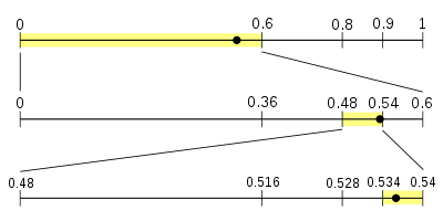
When talking about data compression based on statistical methods, Huffman coding must be mentioned, even though it is a retired champion. The problem with Huffman coding is that the codes have to be an integral number of bits long. For example, if the probability of a character is 1/3, the optimum number of bits to code that character is around 1.6. The Huffman coding scheme has to assign either 1 or 2 bits to the code, and either choice leads to a longer compressed message than is theoretically possible. The image below is a very good illustration for the essence of the thought behind arithmetic coding.
Then the Huffman coding was replaced by the Arithmetic coding, which completely bypasses the idea of replacing an input symbol with a specific code. Instead, it takes a stream of input symbols and replaces it with a single floating point output number. The longer (and more complex) the message, the more bits are needed in the output number. It was not until recently that practical methods were found to implement this on computers with fixed sized registers.
At first glance, the arithmetic coding seems completely impractical, since the floating number with infinite precision is used during the calculation. But most computers only support floating point numbers of up to 80 bits or so. Some high-level programming languages provide support to numbers with infinite precision, such as Fraction and Decimal in Python. However, such supports in the high-level languages are only for ‘simple’ calculation, not for intensive calculations, efficiency and speed are not guaranteed.
In fact, we did implement an arithmetic coding in Python by using rational numbers (Fraction module in Python). The code is really simple and neat indeed. However, even though the efficiency of the algorithm is not the first concern in this project (in order to get the shortest program), the speed for compressing and decompressing is not acceptable at all. The simplicity is at the cost of efficiency.
In practice, we use the fixed-length integer to simulate infinite-precision floating number. The simulation is realized by rescaling the integer interval on the fly during the compression and decompression. Whenever the most significant digit of higher bound and lower bound match, it will never change in the future, then it can be shifted out as one digit in our encoded number. The situation of underflow should also be considered when the higher bound and lower bound begin to converge, but the most significant digit still remain different, such as 59999 and 60001.
Theoretically, the decoder should be something like 'dividing the encoded number by the symbol probability'. In practice, we can't perform an operation like that on a number that could be billions of bytes long. Actually, the decoder accomplishes the job by simulating the procedure in the encoding part.
gzip is another tool used in this project. It is based on the DEFLATE algorithm, which is a combination of LZ77 and Huffman coding. The DEFLATE algorithm is working on a series of blocks, it will produce an optimised Huffman tree customised for each block of data individually. The block sizes are arbitrary, except that non-compressible blocks are limited to 65,535 bytes.Instructions to generate the necessary Huffman tree immediately follow the block header.
Each block consists of two parts: a pair of Huffman code trees that describe the representation of the compressed data part, and a compressed data part. (The Huffman trees themselves are compressed using Huffman encoding.) The compressed data consists of a series of elements of two types: literal bytes (of strings that have not been detected as duplicated within the previous 32K input bytes), and pointers to duplicated strings, where a pointer is represented as a pair <length, backward distance>. The representation used in the "deflate" format limits distances to 32K bytes and lengths to 258 bytes, but does not limit the size of a block, except for uncompressible blocks, which are limited as noted above.
So, from the overview of the DEFLATE algorithm above, we can see that the effect of compression is achieved by:
We are not going to dig into the details of DEFLATE algorithm here. There is abundant information about GZIP and DEFLATE on the internet, you can also check the reference at the end of the report for further reading, if you are interested.
For info.xpm we first tried to produce the image from scratch. The french flag in the background is easily built with a list comprehension in Python.
We then tried to find the font used for the text, but we didnt find a close enough match. The next idea was to encode the exceptions from the flag (the black pixels) using our arithmetic encoder but even if we encoded only the difference to the last line with the arithmetic encoder, the total size was beyond 1kb.
Right at the start we have also tried different existing graphics formats. The png format set us quite a challenge with 553 bytes plus some 200 bytes to convert it to xpm. (png optimizer was used)
Because of the small size of the png-file we didnt bother trying a lot more to make it maybe a few bytes smaller. The total size of <1kb did not justify that.
As we have used it, here comes a short overview of the png standard:
The file starts with an 8 byte fixed header for identification and other purposes. After that, the file is split up in "chunks", each of which has length, type, data and checksum.
The optimized version of our png file only contains these chunks:
The IDAT chunks are the interesing ones in png compression.
As first step in compression, the png encoder tries to use the 2D neighbourhood of a new pixel in order to predict it. For each line the encoder can choose a new encoding method. As the png standard is quite extensive, we only describe the most common one (also probably the only one used in our case). In the following picture the encoder/decoder already knows the green pixels. The current pixel is red while the grey pixels are unknown ones that will be processed later
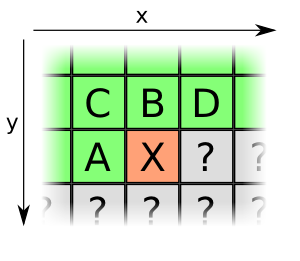
For each pixel the encoder now has the option to encode it using a reference to the pixels A or B, their average, or using the "paeth" with A+B-C. If none of those can be used the compressor will use a reference to the color table in the PLTE chunk. These 5 options are then passed to a DEFLATE compressor which further reduces the the length by using similarities to references seen before.
For more detailed information about the file format refer to the ISO norm or read the short introductory arcticle by one of the creators. Both can be found in the references
The rat.txt file is a string of ones and zeroes which, plotted in 2D, displays a drawing of a rat.
Very soon we realized, that a simple time-independent model would not yield good results because it does not account for the huge white areas around the center. Another idea that we did not implement was runlength encoding. Although it would benefit from the huge white areas, the inner part of the rat is not very optimal for the encoder as short bursts of ones and zeroes dominate.
The first implemented idea was inspired by the good results that png compression yields. As described in the last section, png uses local similarities by creating a lookup table for colors used nearby. Once we looked a little closer we found out that in this case actually a later step of the png compressor (Deflate) yields most gain, but we kept the idea to account for the 2D neighbourhood.
We now ran over the picture and for each pixel we created a histogramm from the neighbourhood that is already known if you would read the file sequentially. This means for pixel with coordinates (x,y), the histogramm is created from [(x-1,y),(x-1,y-1),(x,y-1),(x+1,y-1)]. At the borders we simply wrapped around them to avoid adding more complex code. (The -1th line was assumed to be all white)
This histogramm was actually split into those yielding white and black pixels at (x,y), thus giving us the ability to improve the prediction for the next pixel significantly compared to the time independent approach.
We were not really satisfied with the results, as for example the white surroundings still took up a lot of space (>1/10 bit). To further improve the results we added polygons by hand (done in inkscape). The first one was used to separate the rat from the white background. We experimented with bezier and spline polygons but in the end we took simple line polygons because the extra data needed for the other two was too high compared to the improval in the fit and the additional code needed to draw them.
The 2 regions that can be constructed from the first polygon (inside vs outside) gave us very different results for the histogramms and the encoding improved significantly.
It was then further improved by adding 2 more regions, one with > 95% black pixels and one with > 90% white pixels (approx.)
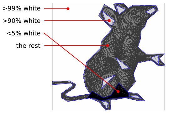 The regions for the rat image. |
different regions and histogramms | ||||||||||||||||||||||||||||||||||||
In the final compression/decompression the probabilites for black and white were hardcoded for each region and for each possible histogramm (i.e. count of white pixels in the known neighbourhood). These probabilites then went straigt to the arithmetic encoder.
 curve1.dat plotted against curve1.sdat | 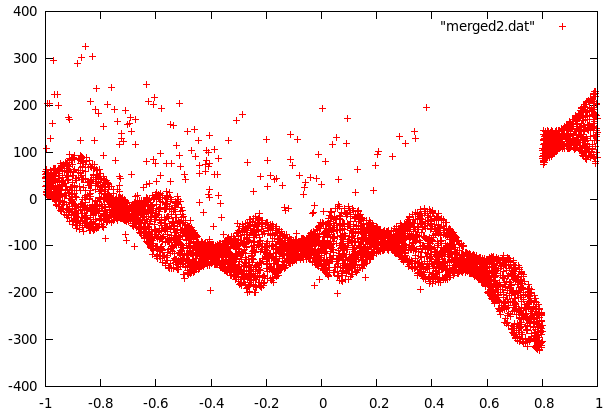 curve2.dat plotted against curve2.sdat |
When sdata is used to plot the curve data, it turns into what seems to be data points scattered around some function for both of the curves. The first step was to approximate these functions so that the scattered data would be centered around the x-axis. This fitting was done in gnuplot and we tried polynomials of different orders.
For curve1 we used 2 functions because of the significant change at x=0.
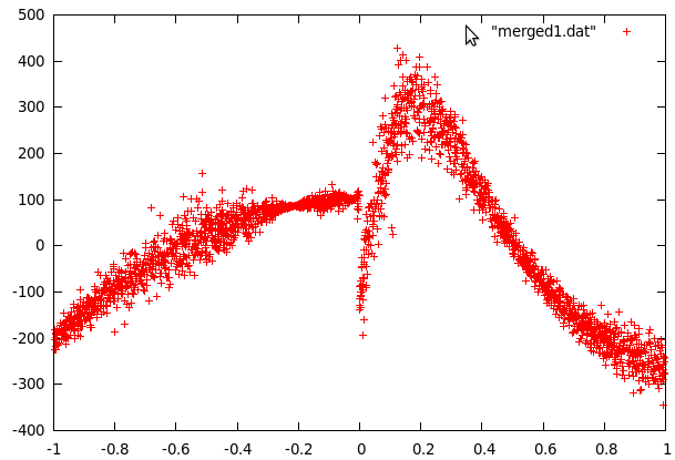
Curve2 was a little more complex because the data contained fairly many far-off values and a strange jump in the values at 0.8. The jump was easy to remove by setting y to -y-180 for all values past this point. To get rid of the far off errors, we first fitted a function to the data and then used the difference to decide if data points were far-off (blue crosses in the following picture) or data from the center. The fitting was then repeated with the points in the center area only (the sine shape was also used to improve the fit).
In both cases fairly few parameters were sufficient to get a good fit.
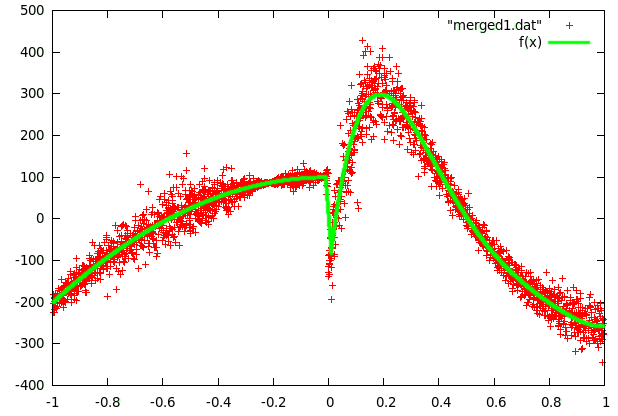 fitting of curve1 - f(x): 3rd and 5th order polynomials combined | 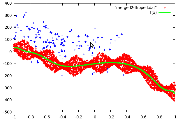 fitting of curve2 - f(x): 12th order polynomial |
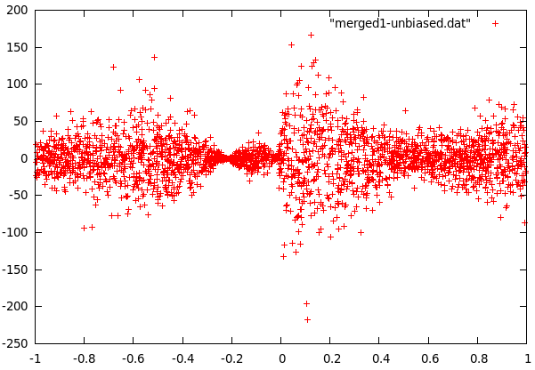 difference of curve1 and f(x) | 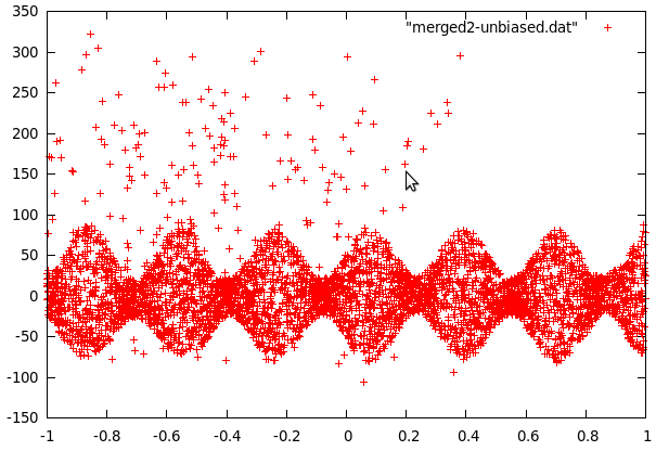 difference of curve2 and f(x) |
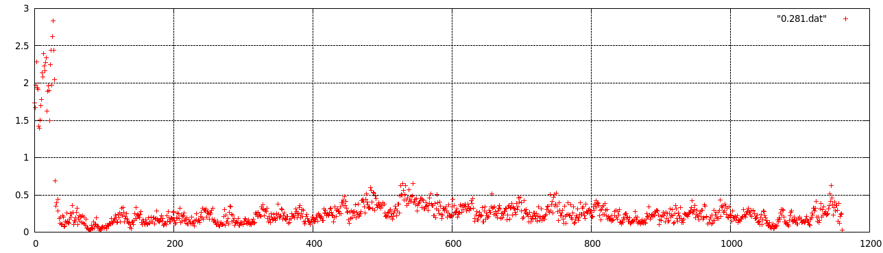
It turns out that the center part of curve2 can be modeled as evenly distributed in an interval whose size is a sine function of x and some sparse errors far off, while curve1 follows a gaussian distribution with a standard deviation that can be approximated with polynomic function of x. The even distribution was relatively easy to build (take y values in a small interval and find maximum of abs but omit far off values). The gaussian first required to calculate the local variance for every data point. This data was then used in gnuplot to fit several polynomials to the variance.
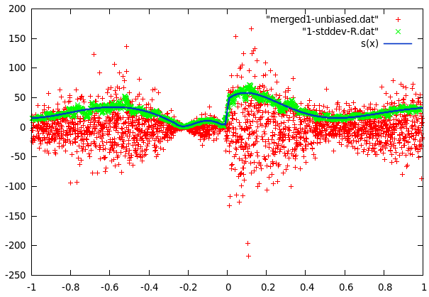 standard deviation of curve1 with function fitted to it | 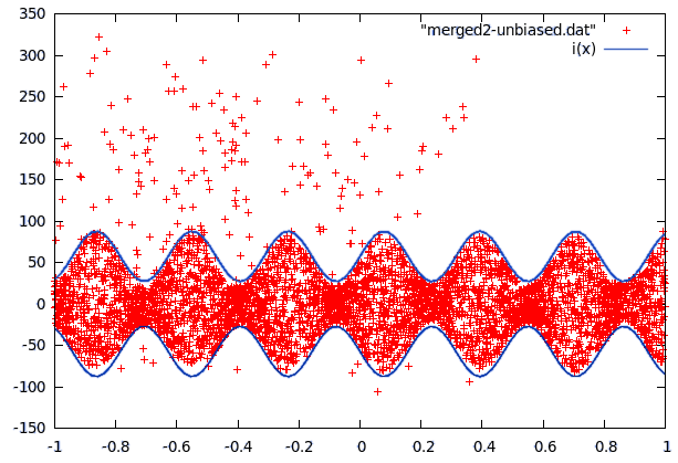 the interval for the euqal distributionof curve2 |
What was left to do now was to study the far-off errors in curve2. It turns out they are relatively frequent if x<-0.35, a little less frequent if x<0.38 and there are no errors past x>0.38. The plot was now divided in 3 mutually exclusive regions: The first one being inside the sine curve, the second one left of -0.35 and the thrid one from -0.35 to 0.38. To cope with local problems with the fitted sine, a fourth area was added. It contains anything within 5 units of the sine.
For each of these regions, we now counted the points and measured the surface it covered to calculate probabilites for a datapoint lying at a certain position in one of these areas. This approach could have been improved (integration), but it would have increased the model size unproportionally.
Equipped with all the parameters for the distribution of a value y for a given x we were now able to compress the curves using the arithmetic encoder.
For the letters task, we had a data file consisting of letters from A to Z and an sdata file containing several attributes of images of the letters. For good compression, we needed to predict the letters from those attributes. So the letter task turns down to be a classification problem with 16-dimensional inputs, 26 classes and 20000 instances.
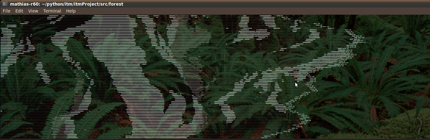
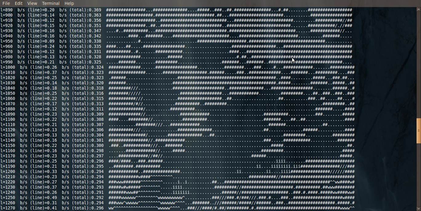
Looking at the data in different editors we noticed that there seems to be a strong influence not just from the preceeding symbol but also from the recently observed patterns. If you change the width of your editor window (word wrap enabled), you come across areas that look like a 2D image. We decided to try this automatically to find the best line width. As it turned out, the optimal line width changes frequently. What we did now is to start with a hand-fitted line length at the beginning of the file. Now we searched for the optimal linewidth w for which another line (w steps fruther down) of the same length w deviates as little as possible from the current one. As the results of this looked very promissing we then switched to not using the .dat part but the .sdat part instead. Of the given values we deemed "elevation" to be most useful to find geographic correlations. We found that using elevation was even more robust than just using forest.dat.
One big problem now was the fact that the length of the lines varied. if we wanted to compare lines to each other we would have had no data available for the end of a line if the previous one was shorter. To cope with this problem we improved the line matching to look for scaled versions of the current line instead of just a very close exact match. The same scaling could then be used to scale the previous line to the length of the current one. We then tried a similar technique as with the rat and the png algorithm of using the local neighbourhood to predict a new "pixel". As the data was a little different we used a bigger area than just the 4-neighbourhood and we gave weights to different spots. Using just this combined with averaged probabilites for each treetype, we were able to push down the size to about 20kb. We tried now to merge the Neural Network with the line predictor, as the errors of each model seemed to have little correlation.
Sadly we were not able to finish this part. From the entropy data we had expected to get below 10kb total size with this approach.
We did not spend much time trying to compress data from the other teams. The only things we tried were 1-10th order Markov chain and looking for similarities to Python's random generator. Neither approach found anything significant so we just left the data in it's original shape.