final.dat
This data consists of data file final.dat and side information file final.sdat. Data file has 20000 floating point numbers separated by new lines and side information contains two floating point numbers for each line in data file. Data and side information was grouped line by line to form a three dimensional space \((X,Y,Z)\). Each data point is then a 3-tuple \((x, y, z)\), where \(x\) contains data to compress and \(y\) and \(z\) the two side information columns.
For closer inspection, the data was plotted in 3D space as is seen in Figure 1. When inspecting the figure, we can see that the data seems to have two distinct shapes, or planes, in it.

Figure 1. Data (\(\,X\,\)) and side information (\(\,Y,Z\,\)) plotted in 3D space.
Note
There is a small side question if the upper shape should be modeled as two shapes in itself, divided by the rip in the shape around \(z = 0.5\); or if the lower plane actually starts from the rip and is somehow mirrored with respect to \(Z\)-axis.
We first tried to fit single plane on the data, but the basic polynomial fitting functions could not handle the sharp curve around the maximum of \(Z\)-dimension. This lead us to an idea to divide the data into two sets using a plane. For optimal dividing plane, we fitted a curve on the data points near the maximum of \(Z\)-dimension (threshold \(0.05\)), which can be seen in Figure 2. Using this curve we can obtain a plane in Figure 3., and split the data into two sets depending if the point is under or above the plane.

Figure 2. Curve fitted to data points near the maximum of \(Z\).

Figure 3. Splitting plane generated from the curve in Figure 2.
Once data was divided, it was easy to fit a single plane into both of the sets using polynomials found from Matlab’s curve fitting tool. We used polynomials of order 5 (probably order 3 would have been sufficient and saved some decompressor size because of fewer coefficients), i.e.
The obtained planes can be seen in Figure 4. and Figure 6., and the residuals between the planes and the data points in Figure 5. and Figure 7.
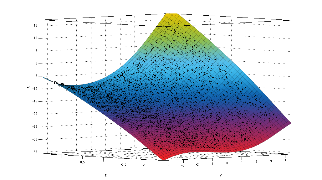
Figure 4. Plane fitted to points under the splitting plane.
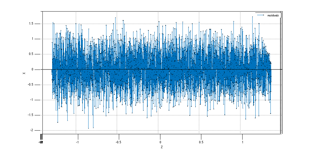
Figure 5. Residuals of data points in question compared to plane in Figure 4.
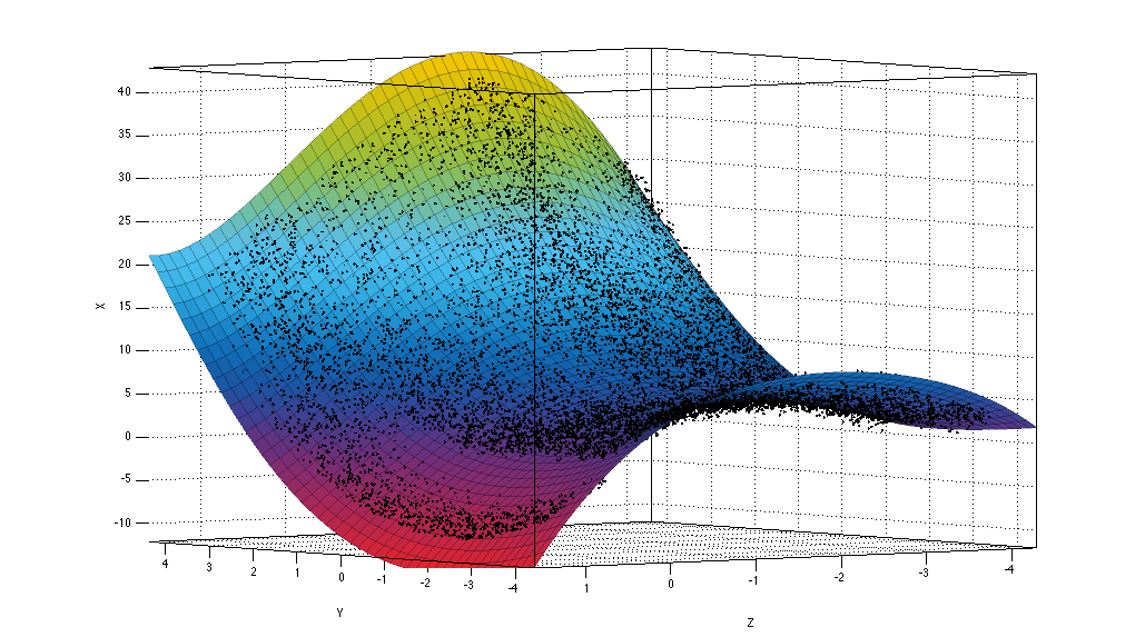
Figure 6. Plane fitted to points above the splitting plane.

Figure 7. Residuals of data points in question compared to plane in Figure 6. The rip in the data around \(z = 0.5\) can be seen in the residuals.
After obtaining the residuals we used mixed model to compress the data: (a) choice between two plane models, sign of a residual and residual’s integer part was grouped together, and (b) the residual’s decimal part was handled separately.
For (a) we used + and - to mark plane models above and below the dividing plane, respectively, and concatenated this information with the sign (also + and -) and the integer part of the residual. With this procedure we obtained strings like +-1 or -+0 for each residual. These strings were then used as individual symbols for Huffman code generation.
For (b) we observed, that the original data was given with floating point precision at most 3. This leads to the fact that storing 3 digits of residual decimals will be sufficient to obtain any of the original data points when combined with the plane model used in calculating the residual – given the side information. We rounded each residual’s decimal part to a fixed floating point precision 3 and concatenated the results as a string, which yielded us a string of length 60000. This string was then Huffman coded using each character, i.e. digits from 0 to 9, as individual symbol.
Finally we added the information of the (symbol, code) -mappings (see Huffman Coding and Decoding for details) into the start of both parts (a) and (b) and concatenated the results to obtain the compressed binary file.