The model

The basic model is the same as the one presented in Section 4.1. The hidden state sequence is denoted by $\boldsymbol{M}= (M_1, \ldots, M_T)$ and other parameters by $\boldsymbol {\theta }$. The exact form of $\boldsymbol {\theta }$ will be specified later. The observations $\boldsymbol{X}= (\mathbf{x}(1), \ldots, \mathbf{x}(T))$, given the corresponding hidden state, are assumed to be Gaussian with diagonal covariance matrix.

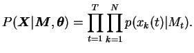
Given the HMM state sequence $\boldsymbol {M}$, the individual observations are assumed to be independent. Therefore the likelihood of the data can be written as

$$P(\boldsymbol{X}\vert \boldsymbol{M}, \boldsymbol{\theta}) = \prod_{t=1}^T \prod_{k=1}^N p(x_k(t) \vert M_t).$$ (5.1)

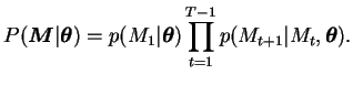
Because of the Markov property, the prior distribution of the probabilities of the hidden states can also be written in factorial form:

$$P(\boldsymbol{M}\vert \boldsymbol{\theta}) = p(M_1 \vert \boldsymbol{\theta}) \prod_{t=1}^{T-1} p(M_{t+1} \vert M_{t}, \boldsymbol{\theta}).$$ (5.2)

The factors of Equations (5.1) and (5.2) are defined to be

$$p(x_k(t) \vert M_t = i) = N(x_k(t);\; m_k(i), \exp(2 v_k(i)))$$ (5.3)

$$p(M_{t+1} = j \vert M_{t} = i, \boldsymbol{\theta}) = a_{ij}$$ (5.4)

$$p(M_1 = i \vert \boldsymbol{\theta}) = \pi_i.$$ (5.5)

The priors of all the parameters defined above are

$$p(\mathbf{a}_{i,\cdot}) = \ensuremath{\text{Dirichlet}}( \mathbf{a}_{i,\cdot};\; \mathbf{u}^{(A)}_i )$$ (5.6)

$$p(\boldsymbol{\pi}) = \ensuremath{\text{Dirichlet}}( \boldsymbol{\pi};\; \mathbf{u}^{(\pi)})$$ (5.7)

$$p(m_k(i)) = N(m_k(i);\; m_{m_k}, \exp(2 v_{m_k}))$$ (5.8)

$$p(v_k(i)) = N(v_k(i);\; m_{v_k}, \exp(2 v_{v_k})).$$ (5.9)

These should be written as conditional distributions conditional to the parameters of the hyperprior but the conditioning variables have been dropped out to simplify the notation.

The parameters $\mathbf{u}^{(\pi)}$ and $\mathbf{u}^{(A)}_i$ of the Dirichlet priors are fixed. Their values should be chosen to reflect true prior knowledge on the possible initial states and transition probabilities of the chain. In our example of speech recognition where the states of the HMM represent different phonemes, these values could, for instance, be estimated from textual data.

All the other parameters $m_{m_k}, v_{m_k}, m_{v_k}$ and $v_{v_k}$ have higher hierarchical priors. As the number of parameters in such priors grows, only the full structure of the hierarchical prior of $m_{m_k}$ is given. It is:

$$p(m_{m_k}) = N(m_{m_k};\; m_{m_{m}}, \exp(2 v_{m_m}))$$ (5.10)

$$p(m_{m_{m}}) = N(m_{m_{m}};\; 0, 100^2)$$ (5.11)

$$p(v_{m_m}) = N(v_{m_m};\; 0, 100^2).$$ (5.12)

The hierarchical prior of for example $\mathbf{m}(i)$ can be summarised as follows:

• The different components of $\mathbf{m}(i)$ have different priors whereas the vectors corresponding to different states of the HMM share a common prior, which is parameterised with $m_{m_n}$.
• The parameters $m_{m_n}$ corresponding to different components of the original vector $\mathbf{m}(i)$ share a common prior parameterised with $m_{m_m}$.
• The parameter $m_{m_m}$ has a fixed noninformative prior.

The set of model parameters $\boldsymbol {\theta }$ consists of all these parameters and all the parameters of the hierarchical priors.

In the hierarchical structure formulated above, the Gaussian prior for the mean $m$ of a Gaussian is a conjugate prior. Thus the posterior will also be Gaussian.

The parameterisation of the variance with $\sigma^2 = \exp(2 v)$, $v \sim N(\alpha, \beta)$ is somewhat less conventional. The conjugate prior for variance of a Gaussian is the inverse gamma distribution. Adding a new level of hierarchy for the parameters of such a distribution would, however, be significantly more difficult. The present parameterisation allows adding similar layers of hierarchy for the parameters of the priors of $m$ and $v$. In this parameterisation the posterior of $v$ is not exactly Gaussian but it may be approximated with one. The exponential function will ensure that the variance will always be positive and the posterior will thus be closer to a Gaussian.