


Assuming
![]() is fixed, the cost function can be written, up to
an additive constant, in the form
is fixed, the cost function can be written, up to
an additive constant, in the form
By defining
The expression
![]() is minimised with
respect to
is minimised with
respect to ![]() by setting
by setting
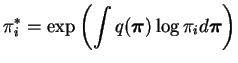
![]() where
where ![]() is
the appropriate normalising constant [39]. This can be
proved with similar reasoning as in Equation (3.13).
is
the appropriate normalising constant [39]. This can be
proved with similar reasoning as in Equation (3.13).
The cost in Equation (6.13) can thus be minimised by setting
The derived optimal approximation is very similar in form to the exact
posterior in Equation (4.6). Therefore the point
probabilities of
![]() and
and
![]() can be
evaluated with a modified forward-backward iteration. The result is
the same as in Equation (4.9) except that in the
iteration,
can be
evaluated with a modified forward-backward iteration. The result is
the same as in Equation (4.9) except that in the
iteration, ![]() is replaced with
is replaced with ![]() ,
, ![]() is replaced
with
is replaced
with ![]() and
and
![]() is replaced with
is replaced with
![]() .
.
![\begin{displaymath}\begin{split}C(\boldsymbol{M}) &= \sum_{\boldsymbol{M}} q(\bo...
...A} + \sum_{t=1}^T C(\mathbf{x}(t) \vert M_t) \bigg] \end{split}\end{displaymath}](img382.gif)
 and
and 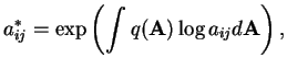
![$\displaystyle C_{q(\boldsymbol{M})} = \sum_{\boldsymbol{M}} q(\boldsymbol{M}) \...
...1}}^* \right] \left[ \prod_{t=1}^T \exp(- C(\mathbf{x}(t) \vert M_t)) \right]}.$](img387.gif)
![$\displaystyle q(\boldsymbol{M}) = \frac{1}{Z_M} \pi_{M_1}^* \left[ \prod_{t=1}^...
...t+1}}^* \right] \left[ \prod_{t=1}^T \exp(- C(\mathbf{x}(t) \vert M_t)) \right]$](img392.gif)