Evaluating the cost function

As before, the general cost function of ensemble learning, as given in Equation (3.11), is

$$\begin{split}C(\boldsymbol{S}, \boldsymbol{\theta}) &= C_q + ... ...mbol{\theta}) - \log p(\boldsymbol{\theta}) \right] \end{split}$$ (6.25)

where the expectations are taken over $q(\boldsymbol{S}, \boldsymbol{\theta})$. This will be the case for the rest of the section unless stated otherwise.

In the NSSM, all the probability distributions involved are Gaussian so most of the terms will resemble the corresponding ones of the CDHMM. For the parameters $\boldsymbol {\theta }$,

$$C_q(\theta_i) = \operatorname{E}\left[ \log q(\theta_i) \right] = -\frac{1}{2} (1 + \log (2 \pi \widetilde{\theta_i})).$$ (6.26)

The term $C_q(\boldsymbol{S})$ is a little more complicated:

$$\begin{split}C_q(\boldsymbol{S}) &= \operatorname{E}\left[ \l... ...\left[ \log q(s_k(t+1) \vert s_k(t)) \right] \Big). \end{split}$$ (6.27)

The first term reduces to Equation (6.26) but the second term is a little different:

$$\begin{multline} E_{q(s_k(t), s_k(t+1))} \left[ \log q(s_k(t+1) \vert s_k(t)) \... ...5ex][0ex]{\ensuremath{\scriptscriptstyle \,\circ}}}{s}}_k(t+1))). \end{multline}$$

The expectation of $- \log p(\theta_i \vert m, v)$ has been evaluated in Equation (6.5), so the only remaining terms are $\operatorname{E}\left[ - \log p(\boldsymbol{X}\vert \boldsymbol{S}, \boldsymbol{\theta}) \right]$ and $\operatorname{E}\left[ - \log p(\boldsymbol{S}\vert \boldsymbol{\theta}) \right]$. They both involve the nonlinear mappings $\mathbf{f}$ and $\mathbf{g}$, so they cannot be evaluated exactly.

The formulas allowing to approximate the distribution of the outputs of an MLP network $\mathbf{f}$ are presented in Appendix B. As a result we get the posterior mean of the outputs $\overline{f}_k(\mathbf{s})$ and the posterior variance, decomposed as

$$\widetilde{f}_k(\mathbf{s}) \approx \widetilde{f}_k^*(\mathbf{s})... ...\widetilde{s}_j \left[ \frac{\partial f_k(\mathbf{s})}{\partial s_j} \right]^2.$$ (6.28)

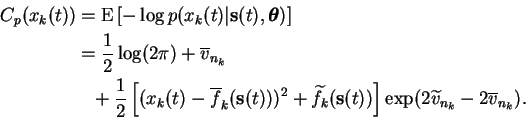
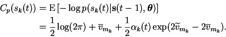
With these results the remaining terms of the cost function are relatively easy to evaluate. The likelihood term is a standard Gaussian and yields

$$\begin{split}C_p(x_k(t)) &= \operatorname{E}\left[ - \log p(x... ... \exp(2\widetilde{v}_{n_k} - 2 \overline{v}_{n_k}). \end{split}$$ (6.29)

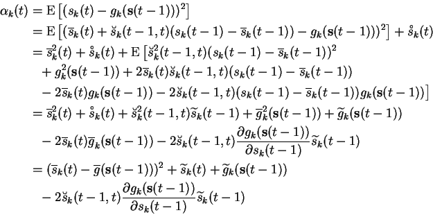
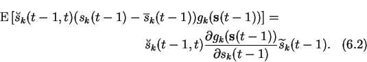
The source term is more difficult. The problematic expectation is

$$\begin{split}\alpha_k(t) &= \operatorname{E}\left[ (s_k(t) - ... ...{s}(t-1))} {\partial s_k(t-1)} \widetilde{s}_k(t-1) \end{split}$$ (6.30)

where we have used the additional approximation

$$\begin{multline} \operatorname{E}\left[ \breve{s}_k(t-1,t) (s_k(t-1) - \overlin... ... g_k(\mathbf{s}(t-1))} {\partial s_k(t-1)} \widetilde{s}_k(t-1). \end{multline}$$

Using Equation (6.31), the remaining term of the cost function can be written as

$$\begin{split}C_p(s_k(t)) &= \operatorname{E}\left[ -\log p(s_... ...\exp(2 \widetilde{v}_{m_k} - 2 \overline{v}_{m_k}). \end{split}$$ (6.31)