Chapter 10 Automatic differentiation and optimisation
Many problems in computational statistics involve search or optimisation of a complicated function over a high dimensional space. These problems can be addressed more efficiently if information of the derivatives or gradients of the function are available as these reveal important information of the local shape of the function.
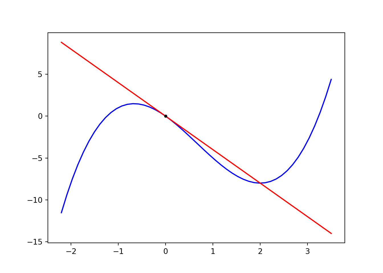
Figure 10.1: Function and its tangent defined by the derivative.
This chapter introduces automatic differentiation which can be used to compute derivatives easily, exactly and efficiently.
Automatic differentiation (autodiff) is at the heart of many modern software libraries and toolkits for machine learning as well as statistics such as TensorFlow, Torch and PyTorch as well as Stan. There is unfortunately no good automatic differentiation toolkit for R at the moment, so one has to use other languages such as Python instead.
10.1 Derivatives of multivariate functions \(f : \mathbb{R}^n \rightarrow \mathbb{R}^m\)
When \(m=1\) and \(n > 1\), the \(n\)-dimensional vector of partial derivatives measuring the change of the function in each coordinate direction is called the gradient and denoted \[ \nabla f(x) = \left( \frac{\partial f}{\partial x_1}, \dots, \frac{\partial f}{\partial x_n} \right). \] Geometrically the gradient is a vector pointing to the direction where the function grows the fastest.
When both \(n,m > 1\), the \(m \times n\) matrix of partial derivatives is called the Jacobian matrix \(\mathbf{J}\), satisfying \[ J_{ij} = \frac{\partial f_i}{\partial x_j}. \] Geometrically the Jacobian matrix defines a mapping which is locally the best linear approximation of \(f\).
When \(m=1\) and \(n > 1\), we can also define an \(n \times n\) matrix \(\mathbf{H}\) of second derivatives called the Hessian matrix, with \[ H_{ij} = \frac{\partial^2 f}{\partial x_i \partial x_j}. \] Geometrically the Hessian matrix defines the curvature of the function at a point, and it is especially important in interpreting the shape of the function when \(\nabla f(x) = 0\).
Gradients and other derivatives of a function are important because they enable efficient optimisation using for example Newton’s method for minimisation of \(f(x)\) through \[ x_{n+1} = x_{n} - \frac{f'(x_{n})}{f''(x_{n})}, \] or in higher dimensional case using \[ x_{n+1} = x_{n} - [Hf(x_{n})]^{-1} \nabla f(x_n), \] or one of numerous proposed simplified variants. Gradient-based optimisation forms the basis for deep learning with neural networks, where the main computational challenge is often efficient evaluation of the gradients of the objective function relative to the network weights.
10.2 Approaches to differentiation of \(f : \mathbb{R}^n \rightarrow \mathbb{R}^m\)
There are three main approaches for differentiation of a function \(f : \mathbb{R}^n \rightarrow \mathbb{R}^m\):
- Numerical differentiation through finite differences \[f'(x) \approx \frac{f(x+h) - f(x)}{h}\]
- Analytic differentiation
- Automatic differentiation
Numerical differentiation provides limited accuracy, and is often quite inefficient in high dimensional problems.
Analytic differentiation requires a lot of manual work, and numerically stable implementation of the results is often non-trivial.
Automatic differentiation provides a very convenient computational solution that is easy, accurate and numerically stable. It can also easily differentiate algorithms such as for or while loops and not just expressions. Its main drawback is that efficient implementation can be challenging, especially when both \(m,n > 1\).
10.3 Different modes of automatic differentiation for \(f : \mathbb{R}^n \rightarrow \mathbb{R}^m\)
There are two different modes of automatic differentiation that are commonly used: forward mode and backward mode.
Forward mode automatic differentiation tracks all derivatives during the forward pass of computations. This can often be implemented using a dual number system that computes both the result of the original computation and its derivatives at the same time. This method only works when \(n\) is very small because otherwise the amount of data that needs to be propagated becomes unmanageable.
Backward mode automatic differentiation works for scalar-valued functions, such as log-probabilities and other objective functions commonly used in statistics and machine learning. It is based on the application of the chain rule and propagating the derivatives backward from the output. In the case of neural networks, the algorithm is the same as the commonly used back-propagation algorithm used to train the networks.
10.4 Automatic differentiation in Python
There are a number of Python packages providing autodiff capabilities. We will consider two relatively broadly applicable packages that are fairly easy to use: Autograd and PyTorch.
10.4.1 Autograd
Autograd builds upon the NumPy interface and for the most part uses the exact same interface. This makes it very easy to use, but on the downside it is research-quality software and not very efficient. Its use is illustrated below.
import autograd.numpy as np
import autograd.numpy.linalg as npl
from autograd import grad

def f(x, a):
    return np.sin(a*x**3 - 2*x**2 - 4*x)

g = grad(f)

t = np.linspace(-2.2, 3.5, 50)

# grad() only works for functions with a scalar value so it cannot be
# used with this this f() when the input is a vector, therefore we
# need a for loop to compute the values
df = np.zeros(t.shape)
for i in range(len(t)):
    df[i] = g(t[i], 1.0)
plt.plot(t, f(t, 1.0), color='b', label=r'$f$')
plt.plot(t, df, color='g', label=r"$f'$")
plt.legend()
plt.show()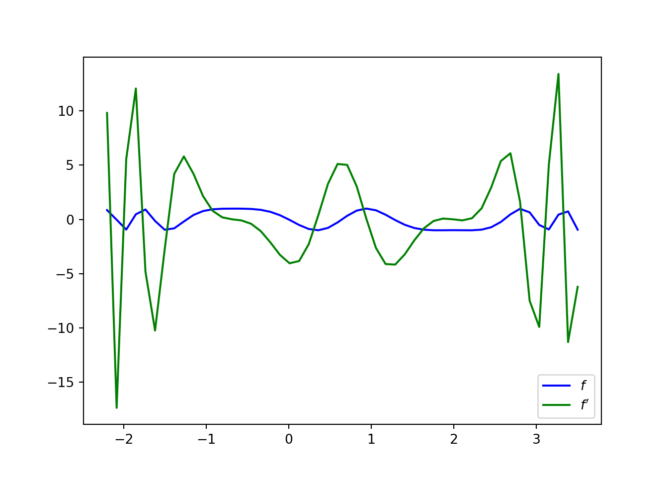
Important autograd features:
- Autograd has a number of sub-packages (
autograd.X) providing wrappers over NumPy and SciPy. It is important to import these instead of standard NumPy and SciPy. autograd.gradalways evaluates the gradient with respect to the first argument, which can be a vector. Other arguments are passed as is.- Autograd can fail if the input
np.arraydata type is integer instead of double or float. This can be avoided by specifying the type manually when constructing arrays or using e.g.1.0instead of1when specifying constants.
10.4.2 PyTorch
PyTorch is a full-fledged deep learning framework with extensive GPU support and other goodies. The interface is a little different from Autograd and the corresponding example is therefore quite a bit more complicated, as seen below.
import torch
import numpy as np
import matplotlib.pyplot as plt

torch.set_default_dtype(torch.double)
# Uncomment this to run on GPU:
# torch.set_default_tensor_type(torch.cuda.DoubleTensor)

def f(x, a):
    return torch.cos(a*x**3 - 2*x**2 - 4*x)

t = torch.linspace(-2.2, 3.5, 50)

# variables used for gradient evaluation are created with requires_grad=True
x = torch.zeros(1, requires_grad=True)

# gradients again need to be evaluated
df = np.zeros(t.shape)
for i in range(len(t)):
    # set the value of the input variable without changing its gradient
    # via .data attribute
    x.data = t[i]
    v = f(x, 1.0)
    # .backward() on function output computes gradients
    v.backward()
    # access gradients via .grad attribute
    df[i] = x.grad
    # gradient needs to be reset before computing the next value
    x.grad.zero_()

# Numpy arrays needed for plotting can be accessed via .numpy()
## tensor(0.)
## tensor(0.)
## tensor(0.)
## tensor(0.)
## tensor(0.)
## tensor(0.)
## tensor(0.)
## tensor(0.)
## tensor(0.)
## tensor(0.)
## tensor(0.)
## tensor(0.)
## tensor(0.)
## tensor(0.)
## tensor(0.)
## tensor(0.)
## tensor(0.)
## tensor(0.)
## tensor(0.)
## tensor(0.)
## tensor(0.)
## tensor(0.)
## tensor(0.)
## tensor(0.)
## tensor(0.)
## tensor(0.)
## tensor(0.)
## tensor(0.)
## tensor(0.)
## tensor(0.)
## tensor(0.)
## tensor(0.)
## tensor(0.)
## tensor(0.)
## tensor(0.)
## tensor(0.)
## tensor(0.)
## tensor(0.)
## tensor(0.)
## tensor(0.)
## tensor(0.)
## tensor(0.)
## tensor(0.)
## tensor(0.)
## tensor(0.)
## tensor(0.)
## tensor(0.)
## tensor(0.)
## tensor(0.)
## tensor(0.)plt.plot(t.numpy(), f(t, 1.0).numpy(), color='b', label=r'$f$')
plt.plot(t.numpy(), df, color='g', label=r"$f'$")
plt.legend()
plt.show()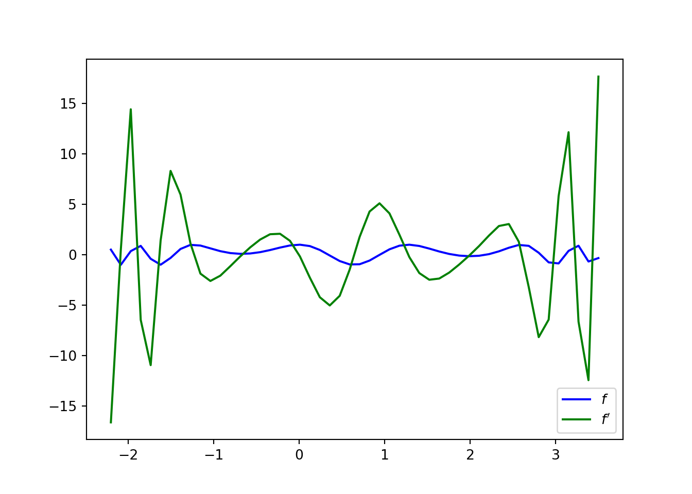
10.5 Gradient-based optimisation methods
Depending on the available computational resources, there are a number of gradient-based optimisation methods. Newton’s method \[ \mathbf{x}_{n+1} = \mathbf{x}_{n} - [\mathbf{H}_{f(\mathbf{x}_{n})}]^{-1} \nabla f(\mathbf{x}_n) \] is the gold standard in accuracy but often computationally too expensive because of the required second-order derivatives and solving a linear system of equations.
Approximations to Newton’s method in decreasing order of convergence speed and memory/iteration cost:
- Quasi-Newton methods approximate the Hessian: BFGS, L-BFGS (limited memory).
- Conjugate gradient methods use conjugate search directions \(s_{n} = -\nabla f(x_n) + \beta_n s_{n-1}\) that guarantee convergence with a quadratic problem in a finite number of steps.
- Gradient descent with plain \(\nabla f(x_n)\).
For general purpose use, BFGS and L-BFGS are often good choices.
10.6 Stochastic gradient optimisation
Many optimisation problems in statistics such as maximum likelihood estimation with independent identically distributed (iid) observations are of the form \[ \min_\theta F(\mathbf{\theta}) = \sum_{i=1}^N f(\mathbf{x}_i, \mathbf{\theta}). \]
When \(N \gg 1\), we can approximate the gradient using a subset of the data \(\{ \mathbf{x}_{s_1}, \dots, \mathbf{x}_{s_M} \}\) \[ \nabla F(\mathbf{\theta}) \approx \frac{N}{M} \sum_{i=1}^M \nabla f(\mathbf{x}_{s_i}, \mathbf{\theta}) =: g(\mathbf{\theta}). \]
Iteratively updating \[ \mathbf{\theta}_{n+1} = \mathbf{\theta}_n - \eta_n g(\mathbf{\theta}_n) \] will converge under mild conditions for \(f\) if (Robbins and Monro (1951)) \[ \sum_{n=1}^\infty \eta_n = \infty, \quad \sum_{n=1}^\infty \eta_n^2 < \infty. \]
10.7 Optimisation with constraints
Many optimisation problems have constraints, such as when optimising the standard deviation \(\sigma\) of the normal distribution, \(\sigma > 0\).
Like with MCMC with constraints, they can be dealt with using specifically designed constrained optimisation algorithms (e.g. L-BFGS-B) or via transformations (e.g. optimise\(\log \sigma\)).
We will focus on transformations because of the connection to MCMC and because they can handle more complex constraints, such as optimising a covariance matrix via Cholesky factors. Transformations in optimisation are typically easier than in MCMC because no density transformations will usually be required.
10.8 Optimisation examples
Let us consider maximum likelihood estimation of the Student’s t-distribution as an example.
Our goal is to estimate the maximum likelihood location parameter and scale parameter of the Student’s t-distribution from observations. Given a data set \(\mathcal{D} = (x_1, \dots, x_n)\), this can be posed s a minimisation problem with the objective \[ f(\mathbf{\theta}) = \sum_{i=1}^n - \log p(x_i | \mathbf{\theta}), \] where the minus sign is needed to turn likelihood maximisation into function minimisation.
In our code we will a 2-component vector \(\mathbf{\theta}\) with the first element denoting the location parameter and the second the log of the scale.
Note: the estimated scale of the Student’s t-distribution is not the same as data standard deviation, and the optimal location parameter is not necessarily the same as the data mean.
10.8.1 Autograd
import autograd.numpy as np
import autograd.numpy.random as npr
import autograd.scipy.stats as sst
import autograd
import scipy.optimize

# Generate a synthetic data set
x = npr.randn(100) + 0.5
print('data mean:', x.mean(), 'data std:', x.std())
## data mean: 0.5689043431805704 data std: 1.0491772219446593def student_logpdf_autograd(x, m, s, nu):
return sst.t.logpdf(x, nu, m, s)
def ltarget(theta):
return -np.sum(student_logpdf_autograd(x, theta[0],
np.exp(theta[1]), 5.0))
g = autograd.grad(ltarget)
theta_opt = scipy.optimize.minimize(ltarget, np.zeros(2),
method='L-BFGS-B', jac = g)
print('location estimate:', theta_opt.x[0],
'scale estimate:', np.exp(theta_opt.x[1]))## location estimate: 0.566070407749397 scale estimate: 0.9281158328110555Notes:
- Autograd does not support named arguments or assignments. Attempting to use them will give mysterious errors.
10.8.2 PyTorch
import torch
import math

torch.set_default_dtype(torch.double)
# Uncomment this to run on GPU:
# torch.set_default_tensor_type(torch.cuda.DoubleTensor)

# Generate a synthetic data set
x = torch.randn(100) + 0.5
print('data mean:', x.mean().item(), 'data std:', x.std().item())
## data mean: 0.5923338160117936 data std: 1.05454491603389def student_logpdf_pytorch(x, m, s, nu):
return torch.distributions.studentT.StudentT(loc=m, scale=s,
df=nu).log_prob(x)
def ltarget(theta):
return -student_logpdf_pytorch(x, theta[0], torch.exp(theta[1]), 5.0).sum()
theta = torch.zeros(2, requires_grad=True)
optimizer = torch.optim.LBFGS([theta])
def closure():
optimizer.zero_grad()
l = ltarget(theta)
l.backward()
return l
optimizer.step(closure)## tensor(161.8564, grad_fn=<NegBackward>)## location estimate: 0.5771483653229711 scale estimate: 0.893293657167386Notes:
- It is important to set the default dtype to
torch.doubleto have sufficient accuracy for statistical computations. Without this setting, all tensors default to single precision floating points which is OK for neural networks but insufficient for statistics. - Some PyTorch functions (e.g. torch.log()) require all arguments to
be tensors created with
torch.tensor(...)instead of scalars or NumPy arrays. - PyTorch BFGS optimiser requires specifying a closure to evaluate the
function value as shown above. Although the optimiser is called
using function
.step(), it actually takes multiple steps up to a specified maximum or convergence. - PyTorch tensors are not pretty when printed.
.item()can be used to extract a single float or.numpy()a NumPy array (except from tensors withrequires_grad=True).
10.9 Literature
Baydin et al. (2018) gives a very comprehensive introduction and history of automatic differentiation in machine learning which closely follows the situation in statistics.
References
Baydin, Atilim Gunes, Barak A. Pearlmutter, Alexey Andreyevich Radul, and Jeffrey Mark Siskind. 2018. “Automatic Differentiation in Machine Learning: A Survey.” Journal of Machine Learning Research 18 (153): 1–43. http://jmlr.org/papers/v18/17-468.html.
Robbins, Herbert, and Sutton Monro. 1951. “A Stochastic Approximation Method.” Ann. Math. Statist. 22 (3): 400–407. https://doi.org/10.1214/aoms/1177729586.