Chapter 2 Simulating pseudorandom numbers

Computers are designed to be deterministic devices. Simulating true randomness on a computer is in general difficult, and most practical applications use pseudorandom numbers—deterministic sequences of numbers that appear random.

Most practical implementations of pseudorandom number generation are based on a random number generator generating uniform random numbers on a suitable subset of integers (often $\{0, \dots, 2^w-1\}$). These numbers can easily be transformed to a uniform distribution over floating point values on the interval $[0,1]$. This uniform pseudorandom number generation in turn serves as a basis for a library of generators for different distributions provided by different statistical software packages and programming languages.

In this chapter we will briefly review the principles these different generators are based upon.

2.1 Uniform pseudorandom number generation

Uniform pseudorandom number generators (PRNGs) form the foundation for any computation requiring randomness.

A good random number generator should have a number of properties:

good statistical properties;
long period before the numbers repeat;
efficient and compact implementation; and
usability in parallel computation.

The most widely used PRNG is Mersenne Twister that combines many of these properties, except it cannot be directly used in parallel computation applications.

The PCG family of PRNGs is gaining popularity as a better alternative that addresses some of the shortcomings of Mersenne Twister. The PCG paper (O’Neill (2014)) provides interesting background reading on modern PRNGs.

2.2 Transformations for non-uniform pseudorandom number generation

Given a uniform PRNG, the simplest way to generate random numbers following a non-uniform distribution is to transform the generated numbers.

For example, an affine transformation of the form $A(x) = ax + b$ can adjust the bounds and scale of a distribution.

The shape of the distribution can be changed using non-linear transformations based on the following theorem:

Theorem 2.1 If $p$ is a random variable with absolutely continuous cumulative density function $\Theta_p(x)$ and $x \sim p$, then \[ \Theta_p(x) \sim \mathrm{Uniform}(0, 1). \]

Applying the inverse transform $\Theta^{-1}_p(y)$ yields the following corollary

Corollary 2.1 Under the assumptions of Theorem 2.1, if $y \sim \mathrm{Uniform}(0, 1)$, then \[\Theta^{-1}_p(y) \sim p. \]

Example distributions where cdf transformation can be used:

exponential distribution
double-exponential distribution a.k.a. Laplace distribution

Example 2.1 Taking an exponentially distributed variable $x \sim \mathrm{Exponential}(\lambda)$ as an example, we have the CDF $\Theta(x) = 1 - \exp(-\lambda x)$ whose inverse is \[\Theta^{-1}(y) = -\frac{\log(1-y)}{\lambda}. \]

Noting that as $y \sim \mathrm{Uniform}(0, 1)$, $y$ and $1-y$ follow the same distribution, we can replace $1-y$ with $y$ to obtain the transformation $-\frac{\log(y)}{\lambda}$.

2.2.1 Generating normally distributed random draws

Normally distributed random variables can be generated using the Box-Muller transformation based on the polar coordinate representation of the bivariate normal distribution.

For $x_1, x_2 \sim N(0, 1)$, \[ p(x_1, x_2) = p(x_1) p(x_2) = \frac{1}{2\pi} \exp( -\frac{x_1^2 + x_2^2}{2}). \]

We can perform a change of variables from $(x_1, x_2)$ to polar coordinates with squared norm as another parameter $(r^2, \theta)$ with \[(x_1, x_2) = (\sqrt{r^2} \cos \theta, \sqrt{r^2} \sin \theta)\].

Using the rule of transformations of probability densities when $\mathbf{y} = f(\mathbf{x})$, \[ p_y(\mathbf{y}) = p_x(f^{-1}(\mathbf{y})) \left| J_{f^{-1}} \right|, \]

we can transform the density. With $f^{-1}(\mathbf{x})$ specified as above, we have \[ J_{f^{-1}} = \begin{pmatrix} -\frac{1}{2\sqrt{r^2}} \cos \theta & -\sqrt{r^2} \sin \theta \\ -\frac{1}{2 \sqrt{r^2}} \sin \theta & \sqrt{r^2} \cos \theta \end{pmatrix}, \] which yields the absolute value of the determinant $\left| J_{f^{-1}} \right| = \frac{1}{2}$.

The transformed probability density is \[ p(r^2, \theta) = \frac{1}{2 \pi} \cdot \frac{1}{2} \exp( -\frac{r^2}{2}), \] which is a product over uniform for $\theta$ and an exponential for $r^2$.

Using two uniform random draws $u_1, u_2$, we can use the cdf transformation to simulate $r^2$ and an affine transformation to simulate $\theta$ as a uniform on the interval $[0, 2 \pi)$. Combining these yields the Box-Muller transform for $(x_1, x_2)$ as \[ (x_1, x_2) = (\sqrt{-2\log u_1} \cos (2 \pi u_2), \sqrt{-2\log u_1} \sin (2 \pi u_2)). \]

2.2.2 Properties of transformation methods:

Transformation methods have guaranteed efficiency, as every input sample is used to generate output.

However deriving the inverse CDF can be difficult or even infeasible for more complicated targets.

2.3 Rejection sampling

Rejection sampling provides a generic alternative for sampling complicated targets for which a transformation required above is not available.

Rejection sampling is based on a geometric idea of drawing samples from a scaled tractable envelope $M \cdot g(x)$ (blue curve in the figure below) that dominates the target distribution $f(x)$ (green curve in the figure below). In order to obtain unbiased samples from $f(x)$, a part of the samples from regions where $M \cdot g(x)$ is large but $f(x)$ is small (the red shaded region in the figure below) need to be rejected and discarded, hence the name. This is achieved by sampling for each proposal $x_i$ an additional $u \sim \mathrm{Uniform}(0,1)$ and only accepting the proposed $x_i$ if $u \cdot M \cdot g(x_i) < f(x_i)$ (the black point falls on the green rather than the red region). (NB: Both $f(x)$ and $g(x)$ need to be normalised probability distributions!)

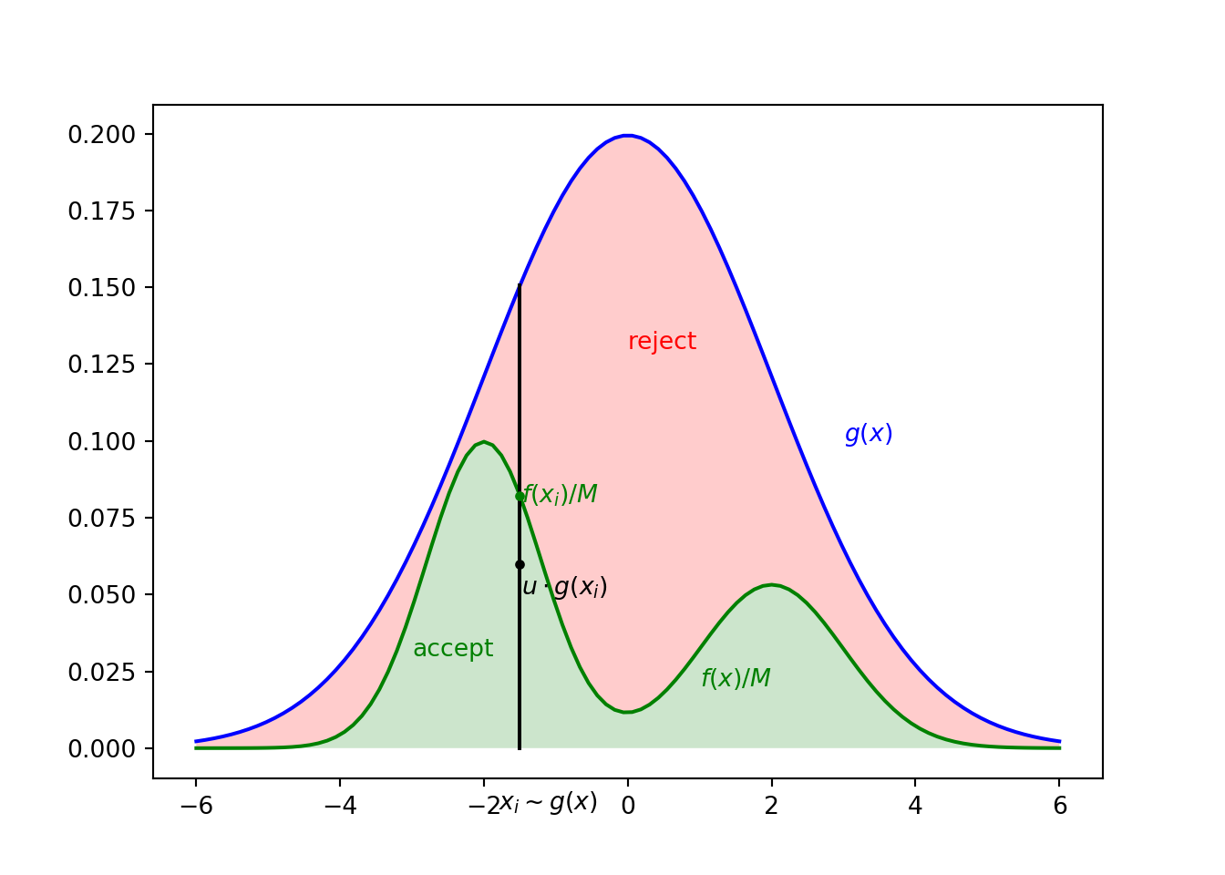
$Illustration of rejection sampling. The proposed point $x_i$ is accepted because $u \cdot g(x_i)$ falls in the green area below $f(x_i) / M$.$

Figure 2.1: Illustration of rejection sampling. The proposed point $x_i$ is accepted because $u \cdot g(x_i)$ falls in the green area below $f(x_i) / M$.

Rejection sampling can be shown to produce samples from the target if $f(x) / M < g(x) \quad \forall x$.

The method is efficient, when $g(x)$ is easy to sample from and as close to $f(x)$ as possible. When both $f(x)$ and $g(x)$ are properly normalised as is assumed, the fraction of samples that are accepted is on average $1/M$.

While rejection sampling is illustrated here for 1D case, it also works for higher dimensional problems, although finding efficient $g(x)$ tends to get more difficult as the dimensionality increases.

Rejection sampling can be implemented as follows:

import numpy as np
import numpy.random as npr
 
def RejectionSampler(f_pdf, g_pdf, g_sample, M, N):
    # Returns N samples following pdf f_pdf() using proposal g(x)
    # with pdf g_pdf() that can be sampled by g_sample()
    # Requirement: f_pdf(x)/M <= g_pdf(x) for all x
    i = 0
    x = np.zeros(N)
    while i < N:
        x_prop = g_sample()
        u = npr.uniform(0, 1)
        if (u * M * g_pdf(x_prop)) < f_pdf(x_prop):
            # Accept the sample and record it
            x[i] = x_prop
            i += 1
    return x

This can be used to draw samples from the above example using:

import numpy as np
import numpy.random as npr
import matplotlib.pyplot as plt
 
# Set the random seed
npr.seed(42)
 
# Define normal pdf
def normpdf(x, mu, sigma):
    return 1/np.sqrt(2*np.pi*sigma**2) * np.exp(-(x-mu)**2 / (2*sigma**2))
 
# Define target pdf as a mixture of two normals
def target_pdf(x):
    return 0.6*normpdf(x, -2, 0.8) + 0.4*normpdf(x, 2, 1)
 
# Define the proposal pdf and a function to sample from it
def proposal_pdf(x):
    return normpdf(x, 0, 2)
 
def sample_proposal():
    return 2*npr.randn()
 
# Define M
M = 3
N = 3000
mysample = RejectionSampler(target_pdf, proposal_pdf, sample_proposal, M, N)
fig, ax = plt.subplots(1, 2)
t = np.linspace(-6, 6, 100)
t2 = np.linspace(-10, 10, 100)
 
# Plot f(x) / (M * g(x)) to verify M is valid (the line should be below 1)
ax[0].plot(t2, target_pdf(t2) / (M*proposal_pdf(t2)))
ax[0].set_title('$f(x) / (M \cdot g(x))$')
ax[1].hist(mysample, 100, density=True)

## (array([0.00332453, 0.        , 0.01329813, 0.0099736 , 0.0099736 ,
##        0.0099736 , 0.02659627, 0.03324533, 0.04654347, 0.049868  ,
##        0.06649067, 0.0299208 , 0.09641147, 0.10306053, 0.12633227,
##        0.14627947, 0.16290213, 0.19282293, 0.1894984 , 0.2293928 ,
##        0.22606827, 0.28590987, 0.28258534, 0.23271734, 0.3889704 ,
##        0.27261174, 0.27593627, 0.349076  , 0.30253254, 0.26596267,
##        0.20612107, 0.2293928 , 0.1795248 , 0.149604  , 0.15292853,
##        0.1097096 , 0.10638507, 0.08643787, 0.08643787, 0.07313973,
##        0.0299208 , 0.05319253, 0.0199472 , 0.0598416 , 0.03324533,
##        0.0398944 , 0.02659627, 0.049868  , 0.04321893, 0.049868  ,
##        0.06649067, 0.08311333, 0.08311333, 0.10306053, 0.12300773,
##        0.09641147, 0.10638507, 0.12633227, 0.15292853, 0.14295493,
##        0.10306053, 0.15292853, 0.15625307, 0.17287573, 0.15292853,
##        0.17620027, 0.11303413, 0.1894984 , 0.12633227, 0.17287573,
##        0.1196832 , 0.13630587, 0.11303413, 0.099736  , 0.1196832 ,
##        0.0897624 , 0.0897624 , 0.07313973, 0.03656987, 0.0299208 ,
##        0.04654347, 0.049868  , 0.0299208 , 0.02327173, 0.01662267,
##        0.01329813, 0.0199472 , 0.01662267, 0.00664907, 0.        ,
##        0.00332453, 0.00332453, 0.00332453, 0.00664907, 0.00664907,
##        0.        , 0.        , 0.        , 0.00332453, 0.00332453]), array([-4.42372382, -4.32345912, -4.22319443, -4.12292973, -4.02266503,
##        -3.92240033, -3.82213563, -3.72187094, -3.62160624, -3.52134154,
##        -3.42107684, -3.32081214, -3.22054745, -3.12028275, -3.02001805,
##        -2.91975335, -2.81948865, -2.71922396, -2.61895926, -2.51869456,
##        -2.41842986, -2.31816516, -2.21790047, -2.11763577, -2.01737107,
##        -1.91710637, -1.81684167, -1.71657698, -1.61631228, -1.51604758,
##        -1.41578288, -1.31551818, -1.21525349, -1.11498879, -1.01472409,
##        -0.91445939, -0.81419469, -0.71393   , -0.6136653 , -0.5134006 ,
##        -0.4131359 , -0.3128712 , -0.21260651, -0.11234181, -0.01207711,
##         0.08818759,  0.18845229,  0.28871698,  0.38898168,  0.48924638,
##         0.58951108,  0.68977578,  0.79004047,  0.89030517,  0.99056987,
##         1.09083457,  1.19109927,  1.29136396,  1.39162866,  1.49189336,
##         1.59215806,  1.69242276,  1.79268745,  1.89295215,  1.99321685,
##         2.09348155,  2.19374625,  2.29401094,  2.39427564,  2.49454034,
##         2.59480504,  2.69506974,  2.79533443,  2.89559913,  2.99586383,
##         3.09612853,  3.19639323,  3.29665792,  3.39692262,  3.49718732,
##         3.59745202,  3.69771672,  3.79798141,  3.89824611,  3.99851081,
##         4.09877551,  4.19904021,  4.29930491,  4.3995696 ,  4.4998343 ,
##         4.600099  ,  4.7003637 ,  4.8006284 ,  4.90089309,  5.00115779,
##         5.10142249,  5.20168719,  5.30195189,  5.40221658,  5.50248128,
##         5.60274598]), <a list of 100 Patch objects>)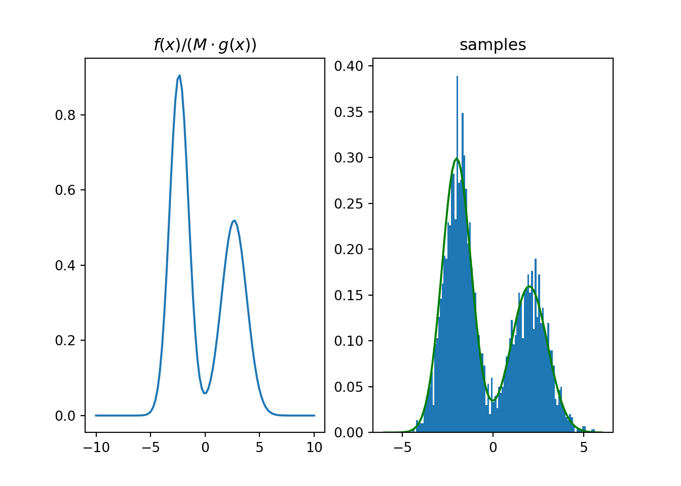

ax[1].plot(t, target_pdf(t), 'g')
ax[1].set_title('samples')
plt.show()

Figure 2.2: Rejection sampling example.

Before applying rejection sampling, it is critical to check that $f(x) / M < g(x) \quad \forall x$. This is checked here by plotting $f(x) / (M \cdot g(x))$ and checking that it remains below 1.

2.4 Inexact methods for non-uniform pseudorandom number generation

Many other methods such as Markov chain Monte Carlo (introduced in Chapter 6) can be used to approximately draw samples from a given distribution.

2.5 Best practices

Make sure you use a good PRNG to avoid strange biases
Be careful when using PRNGs in parallel
Always set and save your random seed to help reproducibility and debugging
… but remember the output may still be different with different hardware and system software etc.
Validate the output of your samplers carefully by testing on a known distribution: sampler errors can be a potential source of very subtle bugs

References

O’Neill, Melissa E. 2014. “PCG: A Family of Simple Fast Space-Efficient Statistically Good Algorithms for Random Number Generation.” HMC-CS-2014-0905. Claremont, CA: Harvey Mudd College. https://www.cs.hmc.edu/tr/hmc-cs-2014-0905.pdf.