Chapter 11 Bayesian model comparison and Laplace approximation
In many inference problems we do not have a single model known beforehand but we want to consider multiple possible models.
Bayesian inference can be applied on a higher level to compare models \(\mathcal{M}_1, \mathcal{M}_2\). The Bayes rule yields \[ p(\mathcal{M}_i | \mathcal{D}) = \frac{p(\mathcal{D} | \mathcal{M}_i) p(\mathcal{M}_i)}{\sum_i p(\mathcal{D} | \mathcal{M}_i) p(\mathcal{M}_i)} \] which depends on the marginal likelihood \[ p(\mathcal{D} | \mathcal{M}_i) = \int_\Theta p(\mathcal{D} | \theta, \mathcal{M}_i) p(\theta | \mathcal{M}_i) \mathrm{d}\theta. \]
Marginal likelihood measures the fit of the model \(\mathcal{M}_i\) to the data \(\mathcal{D}\).
11.1 Model comparison and Bayes factors
Remembering the Bayes rule, we have \[ p(\mathcal{M}_i | \mathcal{D}) = \frac{p(\mathcal{D} | \mathcal{M}_i) p(\mathcal{M}_i)}{\sum_i p(\mathcal{D} | \mathcal{M}_i) p(\mathcal{M}_i)}. \]
Assuming \(p(\mathcal{M}_1) = p(\mathcal{M}_2)\), the posterior odds of the models are given by the ratio of the marginal likelihoods called the Bayes factor \[ B_{12} = \frac{p(\mathcal{M}_1 | \mathcal{D})}{p(\mathcal{M}_2 | \mathcal{D})} = \frac{p(\mathcal{D} | \mathcal{M}_1)}{p(\mathcal{D} | \mathcal{M}_2)} \]
Interpretation (Kass and Raftery (1995))
| \(\log B_{12}\) | Strength of evidence |
|---|---|
| 0 to 1 | not worth more than a bare mention |
| 1 to 3 | positive |
| 3 to 5 | strong |
| >5 | very strong |
11.1.1 Caveats
Bayesian model comparison using model posterior probabilities is theoretically supported only in so-called \(\mathcal{M}\)-closed setting, where the true model is among the considered alternatives (Bernardo and Smith (2001)).
Marginal likelihood is an integral over the prior and as such it is very sensitive to the prior. Changing the prior to cover \(10\times\) larger region in the parameter space e.g. by multiplying the prior standard deviation of a parameter by 10 could cause a 10-fold change in the marginal likelihood while the change in the model posterior and posterior predictions can be minimal.
Despite these weaknesses, marginal likelihood remains a widely used tool for comparing different models.
11.2 Laplace approximation
Laplace approximation provides another common method of approximating the posterior distribution with a Gaussian. The idea stems from so-called Laplace’s method of approximating the integral of a function \(\int f(\theta) d\theta\) by fitting an unnormalised Gaussian at the maximum \(\widehat{\theta}\) of \(f(\theta)\), and computing the volume under the Gaussian. The covariance of the fitted Gaussian is determined by the Hessian matrix of \(\log f(\theta)\) at the maximum point \(\widehat{\theta}\). This can be seen as the second order Taylor approximation of \(\log f(\theta)\).
If \(f(\theta) = p^*(\theta) = p(\mathcal{D}, \theta)\), the approach can be used to evaluate the normaliser of the posterior, i.e. the marginal likelihood.
The same name is also used for the method of approximating the posterior distribution with a Gaussian centered at the maximum a posteriori (MAP) estimate. This can be justified by the fact that under certain regularity conditions, the posterior distribution approaches Gaussian distribution as the number of samples grows.
Laplace approximation is attractive because it is typically very easy to compute, as seen in the example below. It is extremely useful for models where the posterior is indeed Gaussian and can provide a convenient computational shortcut for inference in such models.
Laplace approximation also has a number of important limitations. Obviously it is only suited for unimodal distributions. Like the MAP estimate, it is sensitive to the parametrisation of \(\theta\). Furthermore, if the posterior is skewed in a way that leaves the mode far from the bulk of the posterior mass, Laplace approximation is constrained
Despite using a full distribution to approximate the posterior, Laplace’s method still suffers from most of the problems of MAP estimation. Estimating the variances at the end does not help if the procedure has already lead to an area of low probability mass.
11.3 Marginal likelihood computation
In order to use the Laplace approximation for computing the normalisation constant of a univariate distribution \[ p(\theta) = \frac{p^*(\theta)}{Z} \] such as the marginal likelihood, we use the second order Taylor approximation of \(\log p^*(\theta)\) at the mode \(\widehat{\theta}\): \[ \log p^*(\theta) \approx \log p^*(\widehat{\theta}) - \frac{c}{2} (\theta - \widehat{\theta})^2, \] where the first order term disappears because the derivative is zero at the mode \(\widehat{\theta}\), and \[ c = - \frac{\,\mathrm{d}^2}{\,\mathrm{d} \theta^2} \log p^*(\theta) \bigg\rvert_{\theta = \widehat{\theta}}. \]
The normaliser \(Z\) can now be evaluated as the normaliser or the approximation as \[ Z \approx p^*(\widehat{\theta}) \sqrt{\frac{2\pi}{c}}. \]
In the \(K\)-dimensional multivariate case, the corresponding approximation is \[ \log p^*(\theta) \approx \log p^*(\widehat{\theta}) - \frac{1}{2} (\theta - \widehat{\theta})^T \mathbf{A} (\theta - \widehat{\theta}), \] where \[ A_{ij} = - \frac{\partial^2}{\partial \theta_i \partial \theta_j} \log p^*(\theta) \bigg\rvert_{\theta = \widehat{\theta}} \] is the negative Hessian matrix of \(\log p^*(\theta)\) at \(\widehat{\theta}\).
The normalising constant can now be approximated as \[ Z \approx p^*(\widehat{\theta}) \sqrt{\frac{(2\pi)^K}{\det \mathbf{A}}}. \]
11.4 Example
As an example, we consider evaluating the marginal likelihood in the model of Example 7.1.
Using Autograd to find the posterior mode and evaluate the Hessian, we can approximate the marginal likelihood easily as follows.
import autograd
import autograd.numpy as np
import autograd.numpy.random as npr
import scipy.optimize

def lnormpdf(x, mu, sigma):
    return np.sum(-0.5*np.log(2*np.pi) - np.log(sigma) - 0.5 * (x-mu)**2/sigma**2)

npr.seed(42)
# Simulate n=100 points of normally distributed data about mu=0.5
n = 100
data = 0.5 + npr.normal(size=n)

# Set the prior parameters
sigma_x = 1.0
mu0 = 0.0
sigma0 = 3.0
likelihood = lambda mu: lnormpdf(data, mu, sigma_x)
prior = lambda mu: lnormpdf(mu, mu0, sigma0)

def llikelihood(theta):
    return likelihood(theta) + prior(theta)

def ltarget(theta):
    # note: need to define minimisation separately
    return -llikelihood(theta)

dltarget = autograd.grad(ltarget)
d2ltarget = autograd.hessian(ltarget)

theta_opt = scipy.optimize.minimize(ltarget, np.ones(1),
                                    method='L-BFGS-B', jac = dltarget)
print('posterior mode:', theta_opt.x[0])
## posterior mode: 0.39571380060523365x0 = theta_opt.x[0]
# Z = p*(x0) sqrt(2*pi/c)
# log Z = log p*(x0) + 1/2 log(2pi) - 1/2 log(c)
# Note: taking the absolute value of Hessian to avoid worrying about signs
logZ = llikelihood(x0) + 0.5*np.log(2*np.pi) - 0.5*np.log(np.abs(d2ltarget(x0)))
print("logZ =", logZ)## logZ = -136.1304247617546The same in PyTorch.
import torch
import math
import numpy as np
import numpy.random as npr

torch.set_default_dtype(torch.double)
# Uncomment this to run on GPU
# torch.set_default_tensor_type(torch.cuda.DoubleTensor)

def lnormpdf(x, mu, sigma):
    return torch.distributions.normal.Normal(loc=mu, scale=sigma).log_prob(x).sum()

npr.seed(42)
# Simulate n=100 points of normally distributed data about mu=0.5
n = 100
numpydata = 0.5 + npr.normal(size=n)
data = torch.tensor(numpydata)

# Set the prior parameters
sigma_x = 1.0
mu0 = 0.0
sigma0 = 3.0
likelihood = lambda mu: lnormpdf(data, mu, sigma_x)
prior = lambda mu: lnormpdf(mu, mu0, sigma0)

def llikelihood(theta):
    return likelihood(theta) + prior(theta)

def ltarget(theta):
    # note: need to define minimisation separately
    return -llikelihood(theta)

theta = torch.zeros(1, requires_grad=True)
optimizer = torch.optim.LBFGS([theta])

tol = 1e-6
l_old = math.inf
l_new = ltarget(theta)
while l_old - l_new > tol:
    l_old = l_new
    def closure():
        optimizer.zero_grad()
        l = ltarget(theta)
        l.backward()
        return l
    optimizer.step(closure)
    l_new = ltarget(theta)
## tensor(142.5844, grad_fn=<NegBackward>)
## tensor(134.7462, grad_fn=<NegBackward>)print('posterior mode:', theta[0].item())
# Hessian needs to be computed through repeated gradient evaluation## posterior mode: 0.39571380060523365ll = llikelihood(theta)
def hessian(f, wrt):
g1 = torch.autograd.grad(f, wrt, create_graph=True)[0]
f1 = g1.sum()
return torch.autograd.grad(f1, wrt)[0]
print(hessian(ll, theta))
# Z = p*(x0) sqrt(2*pi/c)
# log Z = log p*(x0) + 1/2 log(2pi) - 1/2 log(c)
# Note: taking the absolute value of Hessian to avoid worrying about signs## tensor([-100.1111])logZ = llikelihood(theta) + 0.5*math.log(2*math.pi) - 0.5*torch.log(torch.abs(hessian(ll, theta)))
print("logZ =", logZ.item())## logZ = -136.130424761754611.5 Marginal likelihood with MCMC using thermodynamic integration
Evaluating marginal likelihood with MCMC is non-trivial. Marginal likelihood is an integral over the prior, but it is usually very heavily dominated by a very small part of the space and hence sampling from the prior to evaluate it results in very high variance of the results.
It is possible to construct an importance sampling estimator to the marginal likelihood as the so called harmonic mean estimator, but this is extremely unreliable in practice and should never be used.
The concept of annealing already considered in Sec. 8.3.2 can also be used to compute the marginal likelihood using a method called thermodynamic integration.
Thermodynamic integration works by drawing samples from \[\pi^*_\beta(\theta) = p(\mathcal{D} | \theta)^\beta p(\theta)\] with \(\beta \in [0, 1]\).
Denoting \[Z_\beta = \int_{\Theta} \pi^*_\beta(\theta) \,\mathrm{d} \theta,\] we have the marginal likelihood \(p(\mathcal{D}) = Z_1\) while \(Z_0 = \int_{\Theta} p(\theta) \,\mathrm{d} \theta = 1\). Let us further denote the normalised distribution \[\pi_\beta(\theta) = \frac{\pi^*_\beta(\theta)}{Z_\beta}. \]
Thermodynamic integration is based on numeric integration \[\ln Z_1 - \ln Z_0 = \int\limits_0^1 \frac{\partial \ln Z_\beta}{\partial \beta} \,\mathrm{d} \beta.\] The required integrand can be evaluated as \[\begin{align*} \frac{\partial \ln Z_\beta}{\partial \beta} &= \frac{1}{Z_\beta} \frac{\partial Z_\beta}{\partial \beta} \\ &= \frac{1}{Z_\beta} \frac{\partial}{\partial \beta} \int_{\Theta} \pi^*_\beta(\theta) \,\mathrm{d} \theta \\ &= \frac{1}{Z_\beta} \int_{\Theta} \frac{\partial \pi^*_\beta(\theta)}{\partial \beta} \,\mathrm{d} \theta \\ &= \int_{\Theta} \frac{1}{\pi^*_\beta(\theta)} \frac{\partial \pi^*_\beta(\theta)}{\partial \beta} \frac{\pi^*_\beta(\theta)}{Z_\beta} \,\mathrm{d} \theta \\ &= \int_{\Theta} \frac{\partial \ln \pi^*_\beta(\theta)}{\partial \beta} \pi_\beta(\theta) \,\mathrm{d} \theta. \end{align*}\] Noting that \[\ln \pi^*_\beta(\theta) = \beta \ln p(\mathcal{D} | \theta) + \ln p(\theta),\] we have \[\frac{\partial \ln \pi^*_\beta(\theta)}{\partial \beta} = \ln p(\mathcal{D} | \theta).\] The integral can be seen as an expectation over \(\pi_\beta(\theta)\). Using the samples from this distribution, we can now evaluate the log-marginal-likelihood as \[\ln p(\mathcal{D}) = \ln Z_1 - \ln Z_0 = \int_0^1 \mathrm{E}_\beta [\ln p(\mathcal{D} | \theta)] \,\mathrm{d}\beta, \] where \(\mathrm{E}_\beta[ \cdot ]\) is an expectation over the annealed posterior \(\pi_\beta(\theta)\) which can be evaluated using Monte Carlo samples from the corresponding chain.
11.6 Thermodynamic integration example
As an example, we will evaluate the marginal likelihood in the model of Example 7.1 that was evaluated using Laplace approximation above.
import scipy.integrate

def lnormpdf(x, mu, sigma):
    return np.sum(-0.5*np.log(2*np.pi) - np.log(sigma) - 0.5 * (x-mu)**2/sigma**2)

npr.seed(42)
# Simulate n=100 points of normally distributed data about mu=0.5
n = 100
data = 0.5 + npr.normal(size=n)

# Set the prior parameters
sigma_x = 1.0
mu0 = 0.0
sigma0 = 3.0

likelihood = lambda mu: lnormpdf(data, mu, sigma_x)
prior = lambda mu: lnormpdf(mu, mu0, sigma0)

CHAINS = 20
ITERS = 10000
betas = np.concatenate((np.array([0.0]), np.logspace(-5, 0, CHAINS)))

xx = np.zeros((ITERS, CHAINS+1))
for i in range(CHAINS+1):
    xx[:,i] = mhsample1(np.zeros(1), ITERS, lambda x: betas[i]*likelihood(x)+prior(x),
                        lambda x: x + 0.2/np.sqrt(betas[i]+1e-3)*npr.normal(size=1))
## Sampler acceptance rate: 0.492
## Sampler acceptance rate: 0.4794
## Sampler acceptance rate: 0.4867
## Sampler acceptance rate: 0.4808
## Sampler acceptance rate: 0.4816
## Sampler acceptance rate: 0.4819
## Sampler acceptance rate: 0.4891
## Sampler acceptance rate: 0.4903
## Sampler acceptance rate: 0.4849
## Sampler acceptance rate: 0.4908
## Sampler acceptance rate: 0.4958
## Sampler acceptance rate: 0.4887
## Sampler acceptance rate: 0.4917
## Sampler acceptance rate: 0.4935
## Sampler acceptance rate: 0.5009
## Sampler acceptance rate: 0.4897
## Sampler acceptance rate: 0.498
## Sampler acceptance rate: 0.4979
## Sampler acceptance rate: 0.5053
## Sampler acceptance rate: 0.4946
## Sampler acceptance rate: 0.4967lls_ti = np.zeros(xx.shape)
for i in range(lls_ti.shape[0]):
for j in range(lls_ti.shape[1]):
lls_ti[i,j] = likelihood(xx[i,j])
ll = np.mean(lls_ti, 0)
plt.plot(betas, ll)
plt.xlabel(r'$\beta$')
plt.ylabel(r'$E_\beta[ \log p(\mathcal{D} | \theta)]$')
plt.show()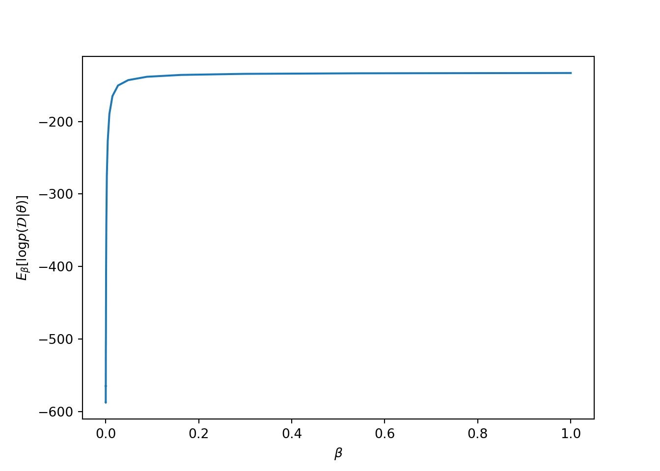
## Marginal likelihood: -136.0731258132228711.7 Notes
Thermodynamic integration can be very naturally combined with parallel tempering because they both require simulating the same annealed distributions \(\pi_\beta(\theta)\).
11.8 Exercises
- Compute the exact marginal likelihood in the example and compare it with the obtained result.
11.9 Literature
Lartillot and Philippe (2006) provide a nice introduction to thermodynamic integration.
References
Bernardo, José M, and Adrian FM Smith. 2001. Bayesian Theory. IOP Publishing.
Kass, R. E., and A. E. Raftery. 1995. “Bayes Factors.” Journal of the American Statistical Association 90: 773–95. https://doi.org/10.1080/01621459.1995.10476572.
Lartillot, Nicolas, and Hervé Philippe. 2006. “Computing Bayes Factors Using Thermodynamic Integration.” Systematic Biology 55 (2): 195–207. https://doi.org/10.1080/10635150500433722.