Chapter 8 MCMC diagnostics and sampling multimodal distributions
8.1 MCMC diagnostics
It is in general impossible to prove that a MCMC chain would have converged, but a number of diagnostics have been developed that can detect if it has not converged.
In addition to convergence, the efficiency of the sampler is often of great interest as this can vary a lot, ranging from reasonably fast to uselessly slow. As all theoretical guarantees of MCMC are asymptotic, efficiency can make a huge difference in how useful the results will be.
8.1.1 Convergence diagnostics
In short, MCMC converge checking is based on starting \(m\) chains from widely dispersed starting points and checking that they end up producing similar results.
The similarity of the results is commonly measured by the potential scale reduction \(\hat{R}\) or R-hat, that measures the factor by which the scale of the current distribution might be reduced if the simulations were continued until \(n \rightarrow \infty\) (Gelman et al. (2013)). \(\hat{R}\) was first introduced by (Gelman and Rubin (1992)) and has been since refined. The estimate of \(\hat{R}\) is based on the within-chain variance \(W\) and between-chains variance \(B\).
Assuming \(\theta_{ij}\) is the \(i\)th sample (out of \(n\)) from chain \(j\) (out of \(m\)), we can define \[ B = \frac{n}{m-1} \sum_{j=1}^m (\theta_{: j} - \theta_{::})^2, \text{ where } \theta_{: j} = \frac{1}{n} \sum_{i=1}^n \theta_{ij}, \theta_{::} = \frac{1}{m} \sum_{j=1}^m \theta_{: j} \] \[ W = \frac{1}{m} \sum_{j=1}^m s_j^2, \text{ where } s_j^2 = \frac{1}{n-1} \sum_{i=1}^n (\theta_{ij} - \theta_{: j})^2. \]
Using these, we can estimate the variance of \(\theta\) as \[ \operatorname{Var}(\theta) = \frac{n-1}{n} W + \frac{1}{n} B. \]
\(\hat{R}\) can now be defined as (Gelman et al. (2013)) \[ \hat{R} = \sqrt{\frac{\mathrm{Var}(\theta)}{W}}. \]
\(\hat{R}\) is defined for scalar variables. For vectors it is common to compute it for each component and take the maximum over different components.
\(\hat{R}\) approaches \(1\) as the \(n\) increases. The threshold of 1.1 is commonly used to consider a chain as having converged.
The original proposal applied \(\hat{R}\) to entire chains. This was later found to sometimes miss cases where the chains are non-stationary, and the current best practice is to split the chains to two halves and consider these as independent chains in the computation, which is sometimes referred to as split-\(\hat{R}\).
8.1.2 Diagnostics of sampling efficiency
The efficiency of MCMC samplers is typically evaluated using autocorrelations of the samples, which measure the correlation of neighbouring samples after a given lag \(k\). The motivation for using autocorrelation is that an optimally efficient sampler would typically produce essentially uncorrelated samples while for an inefficient sampler that makes very small steps, nearby samples would be very highly correlated. Such correlated samples obviously provide less information of the target distribution. Autocorrelations can be conveniently summarised using the effective sample size (ESS), which is a measure of how many independent samples a given sample is worth.
Autocorrelation \(\rho_k\) of a wide-sense stationary process \(\theta_1, \theta_2, \dots\) with lag \(k\) is defined as \[\begin{equation} \rho_k = \frac{E[(\theta_i - \mu)(\theta_{i+k} - \mu)]}{\sigma^2}, \quad k = 0, 1, 2, \dots, \tag{8.1} \end{equation}\] where the expectation is taken over the time index \(i\), \(\mu\) is the mean and \(\sigma^2\) the variance of the process.
Given these autocorrelations, the effective sample size (ESS) for \(M\) samples is defined as \[\begin{equation} \mathrm{ESS} = \frac{M}{1 + 2 \sum_{k=1}^{\infty} \rho_k}. \tag{8.2} \end{equation}\] Clearly uncorrelated samples (\(\rho_k = 0 \;\; \forall k > 0\)) result in \(\mathrm{ESS} = M\) while highly correlated samples result in a very small ESS, confirming the ESS follows the above intuitions about autocorrelations.
While the definitions of Eq. (8.1) and (8.2) may look straightforward, they can be difficult to apply in practice. Especially the estimation of \(\rho_k\) for long lags \(k\) can be unreliable. Unreliable estimates of \(\mu\) and \(\sigma^2\) often lead to significantly negative estimates of \(\rho_k\), which can give unreasonably high ESS estimates.
One recommended way (Geyer (1992)) to moderate the problems with large lags is to use divisor \(1/n\) in the estimate of the autocorrelation from a finite sequence of length \(n\), \(\theta_1, \dots, \theta_n\), although the sum for \(\rho_k\) only has \(n-k\) terms. This effectively shrinks terms with large \(k\) toward 0 and results in estimate \[\begin{equation} \hat{\rho}_k = \frac{1}{n \sigma^2} \sum_{i=1}^{n-k} (\theta_i - \mu)(\theta_{i+k} - \mu), \quad k = 0, 1, 2, \dots. \tag{8.3} \end{equation}\]
Another best practice for avoiding problems arising from bad \(\rho_k\) estimates is to truncate the sum in the denominator of Eq. (8.2) (Gelman et al. (2013)). The sum of pairs \(\rho_{2k} + \rho_{2k+1}\) is known to be positive. This can be used to detect when the \(\rho_k\) estimates become too unreliable and setting the upper bound of the summation to the first odd positive integer \(K\) for which \(\rho_{K+1} + \rho_{K+2}\) is negative. Thus the computation of ESS for \(M\) samples reduces to \[\begin{equation} \widehat{\mathrm{ESS}} = \frac{M}{1 + 2 \sum_{k=1}^{K} \rho_k}, \tag{8.4} \end{equation}\] where \(K\) is as defined above, i.e. \(K = \min \{ j \mid j = 2l+1, l \in \mathbb{N}, \rho_{j+1} + \rho_{j+2} < 0 \}\).
8.2 Good practices for MCMC sampling
- Running three or more chains starting from very different points allows checking convergence.
- Samples from an initial warm-up or burn-in period (e.g. first 50% of samples) are discarded as they depend too much on the initial point.
- The proposal often needs to be tuned to get fast mixing. You should first perform any tuning, then discard all those samples and run the actual analysis. Note that the optimal tuning for warm-up and stationary phases might be different.
- Check for convergence by comparing the chains using e.g. the \(\hat{R}\) statistic.
- Mix the non-warm-up samples from all chains for final analysis.
- Compare your inferences with results from simpler models or approximations.
Gelman and Shirley (2011)
8.3 Improving MCMC convergence
In this section we will introduce general techniques for improving MCMC convergence.
8.3.1 Blocking for high-dimensional distributions
Acceptance rates for proposals naturally go down as the dimensionality of the problem increases. If a scalar proposal has a probability \(p\) of being accepted, \(d\) independent such proposals will have the probability \(p^d\).
One way to counter this trend is by blocking the updates by dividing the parameters to subsets and updating each subset alone in turn. As long as the proposals for each block are reasonable, this will provide a convergent sampler.
The Gibbs sampler implements an extreme form of blocking where each variable is updated in turn. Combining this with a proposal from the conditional posterior of the corresponding variable yields a 100% acceptance rate.
While blocking can help increase acceptance rates, it can lead to inefficient sampling if variables in different blocks are strongly correlated.
8.3.2 Parallel tempering for MCMC for multimodal distributions
Sampling multimodal distributions with MCMC is hard. A successful sampler would need to combine small-scale local exploration with large global jumps between different modes, which are usually incompatible goals.
Parallel tempering methods can greatly speed up MCMC convergence in multimodal distributions. Their basic idea is to run several MCMC chains in parallel. Each chain runs in a different temperature, smoothing out the targets of the “hot” chains, allowing easier exploration. Furthermore a new move for swapping states between the chains is introduced. This allows propagating the results of the fast exploration in the hot chains all the way to the coldest chain that samples the actual target.
Mathematically, instead of sampling a single target \(\pi(\theta)\), we sample \(\pi(\theta)^\beta\) for a range of values \(0 \le \beta \le 1\). In the physics analogue, \(\beta\) is the inverse temperature \(\beta = 1/T\). This provides a smooth transition from the actual target at \(\beta = 1\) to a uniform distribution at \(\beta = 0\). In the context of Bayesian models, the tempering is often applied only to the likelihood term, in which case \[ \pi_{\beta}(\theta) = p(\theta) p(\mathcal{D} | \theta)^\beta. \]
Given a set of temperature values \(B = (\beta_1=1, \dots, \beta_b=0)\), we can define an augmented system over \[ \Theta = (\theta^{(1)}, \dots, \theta^{(b)}) \] with \[ \pi(\Theta) = \prod_{i=1}^b \pi_{\beta_i}(\theta^{(i)}). \]
Following the blocking approach, we introduce a sequence of proposals that are considered and accepted/rejected in sequence:
- Standard MH proposals for each \(\pi_{\beta_i}(\theta^{(i)})\).
- A proposal to swap the states of neighbouring chains.
When considering swapping the states of chains \((i, i+1)\), the acceptance probability for the move is \[ a = \frac{\pi_{\beta_i}(\theta^{(i+1)}) \pi_{\beta_{i+1}}(\theta^{(i)})} {\pi_{\beta_i}(\theta^{(i)}) \pi_{\beta_{i+1}}(\theta^{(i+1)})}. \]
8.3.3 Parallel tempering example
Let us consider parallel tempering with a multimodal target \[ \pi(\theta) = \exp(-\gamma(\theta^2 - 1)^2). \] The target clearly has two modes at \(\theta = \pm 1\). The depth of the valley between the modes is controlled by the parameter \(\gamma\). Setting \(\gamma = 64\) gives highly separated modes that cannot be easily sampled using standard MH sampling, as seen below in Fig. 8.1.
import scipy.integrate

def ltarget(theta, gamma):
    return -gamma*(theta**2-1)**2

# Find the normaliser of the target for visualisation
Z = scipy.integrate.quad(lambda theta: np.exp(ltarget(theta, 64.0)), -2, 2)

npr.seed(42)
theta = mhsample1(1.0, 10000, lambda theta: ltarget(theta, 64.0),
              lambda theta: theta + 0.1*npr.normal())
## Sampler acceptance rate: 0.473theta = theta[len(theta)//2:]
h = plt.hist(theta, 50, density=True)
t = np.linspace(-1.2, 1.2, 200)
plt.plot(t, np.exp(ltarget(t, 64.0)) / Z[0])
plt.show()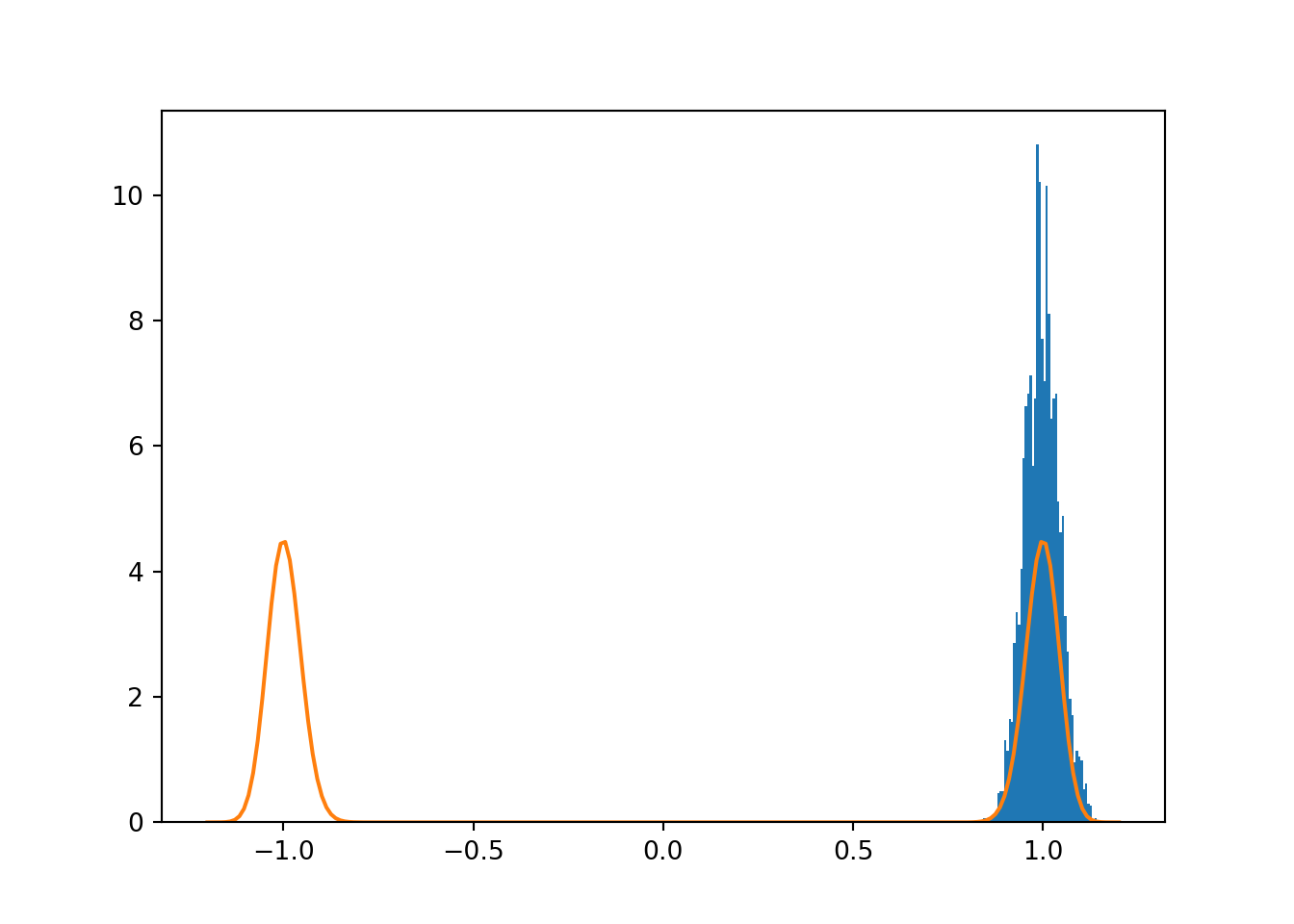
Figure 8.1: Trying to sample a multimodal target using MH sampling.
## 0.996830738176979Parallel tempering can sample this very challenging target with ease, as seen in Fig. 8.3. Here we have used 5 chains with logarithmically spaced \(\beta\) values in the range \([10^{-3}, 1]\) generated using
## [0.001 0.00562341 0.03162278 0.17782794 1. ]The optimal \(\beta\) values should allow for uniform acceptance of swaps between all neighbouring values. This is achieved by having a tighter spacing near 0, as in this example.
The corresponding densities for different \(\beta\) are illustrated in Fig. 8.2.
import scipy.integrate

def ltarget(theta, gamma):
    return -gamma*(theta**2-1)**2

t = np.linspace(-3, 3, 200)
for b in betas:
    # Find the normaliser of the target for visualisation
    Z = scipy.integrate.quad(lambda theta: np.exp(b * ltarget(theta, 64.0)), -4, 4)
    plt.plot(t, np.exp(b * ltarget(t, 64.0)) / Z[0], label=r"""$\beta = %.3f$""" % b)
plt.legend()
plt.show()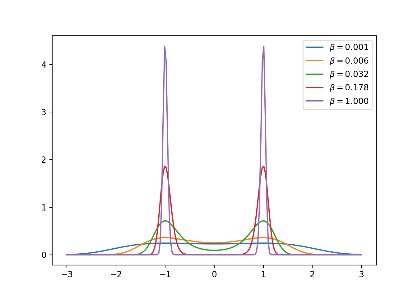
Figure 8.2: Tempered target distributions in the parallel tempering example.
The remaining challenge is to tune the samplers for each \(\beta\) to achieve a good acceptance. In this example this is achieved using a normal proposal \[q_\beta(\theta';\; \theta) = \mathcal{N}(\theta';\; \theta, \sigma_{\text{prop}, \beta}^2)\] with \[ \sigma_{\text{prop}, \beta}^2 = \frac{1}{\beta} 0.1^2, \] which works well for this example. This scaling might cause problems if smaller \(\beta\) values were used.
The trace plots of each \(\beta\) are shown in Fig. 8.4.
def pt_target(theta, beta, gamma):
    return beta * ltarget(theta, gamma)

def pt_msample(theta0, n, betas, target, drawproposal):
    CHAINS = len(betas)
    accepts = np.zeros(CHAINS)
    swapaccepts = np.zeros(CHAINS-1)
    swaps = np.zeros(CHAINS-1)
    # All variables are duplicated for all the chains
    theta = theta0 * np.ones(CHAINS)
    lp = np.zeros(CHAINS)
    thetas = np.zeros((n, CHAINS))
    for j in range(CHAINS):
        lp[j] = target(theta[j], betas[j])
    for i in range(n):
        # Independent moves for every chain, MH acceptance
        for j in range(CHAINS):
            theta_prop = drawproposal(theta[j], betas[j])
            l_prop = target(theta_prop, betas[j])
            if np.log(npr.rand()) < l_prop - lp[j]:
                theta[j] = theta_prop
                lp[j] = l_prop
                accepts[j] += 1
        # Swap move for two chains, MH acceptance:
        j = npr.randint(CHAINS-1)
        h = target(theta[j+1],betas[j])+target(theta[j],betas[j+1]) - lp[j] - lp[j+1]
        swaps[j] += 1
        if np.log(npr.rand()) < h:
            # Swap theta[j] and theta[j+1]
            temp = theta[j]
            theta[j] = theta[j+1]
            theta[j+1] = temp
            lp[j] = target(theta[j], betas[j])
            lp[j+1] = target(theta[j+1], betas[j+1])
            swapaccepts[j] += 1
        thetas[i,:] = theta
    print('Acceptance rates:', accepts/n)
    print('Swap acceptance rates:', swapaccepts/swaps)
    return thetas

npr.seed(42)
betas = np.logspace(-3, 0, 5)
theta = pt_msample(1.0, 10000, betas,
                   lambda theta, beta: pt_target(theta, beta, 64.0),
                   lambda theta, beta: theta + 0.1/np.sqrt(beta)*npr.normal())
## Acceptance rates: [0.4698 0.637 0.5694 0.4845 0.4563]
## Swap acceptance rates: [0.74561404 0.63706096 0.4660707 0.4945184 ]theta = theta[len(theta)//2:]
h = plt.hist(theta[:,-1], 50, density=True)
t = np.linspace(-1.2, 1.2, 200)
plt.plot(t, np.exp(ltarget(t, 64.0)) / Z[0])
plt.show()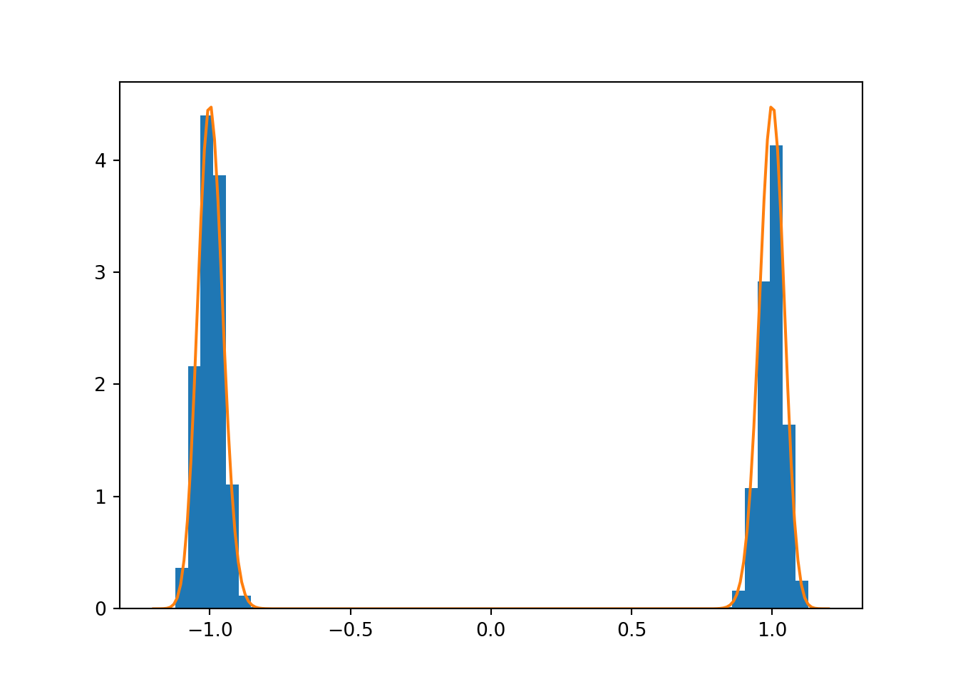
Figure 8.3: Sampling a multimodal target using parallel tempering.
## -0.08167086471587666N = len(betas)
fix, ax = plt.subplots(N, 1, figsize=[6.4, 9.6])
for i in range(N):
ax[i].set_title('beta = %.2f' % betas[i])
ax[i].plot(theta[:,i])
plt.subplots_adjust(hspace=0.4)
plt.show()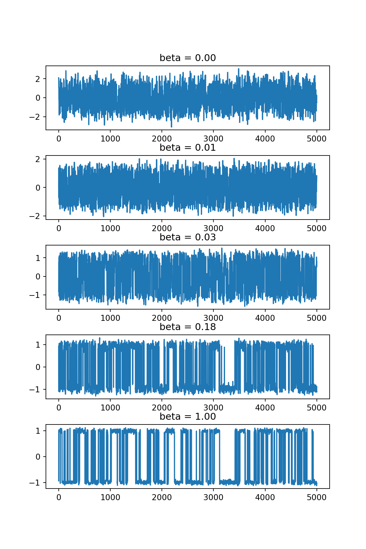
Figure 8.4: Trace plots of parallel tempering chains
8.4 Literature
Koistinen (2013) provides a nice introduction to MCMC theory for the more mathematically inclined readers.
Gelman et al. (2013) present a very through discussion on MCMC diagnostics.
Altekar et al. (2004) present a version of parallel tempering with application to phylogenetic inference.
References
Altekar, Gautam, Sandhya Dwarkadas, John P. Huelsenbeck, and Fredrik Ronquist. 2004. “Parallel Metropolis Coupled Markov Chain Monte Carlo for Bayesian Phylogenetic Inference.” Bioinformatics 20 (3): 407–15. https://doi.org/10.1093/bioinformatics/btg427.
Gelman, Andrew, John Carlin, Hal Stern, David Dunson, Aki Vehtari, and Donald Rubin. 2013. Bayesian Data Analysis. 3rd ed. Boca Raton, FL: Chapman & Hall/CRC.
Gelman, Andrew, and Donald B. Rubin. 1992. “Inference from Iterative Simulation Using Multiple Sequences.” Statistical Science 7 (4): 457–72. https://doi.org/10.1214/ss/1177011136.
Gelman, Andrew, and Kenneth Shirley. 2011. “Inference and Monitoring Convergence.” In Handbook of Markov Chain Monte Carlo, edited by Steve Brooks, Andrew Gelman, Galin Jones, and Xiao-Li Meng. Chapman & Hall/CRC. http://www.mcmchandbook.net/HandbookChapter6.pdf.
Geyer, Charles J. 1992. “Practical Markov Chain Monte Carlo.” Statistical Science 7 (4): 473–83. https://doi.org/10.1214/ss/1177011137.
Koistinen, Petri. 2013. “Computational Statistics.”