Chapter 4 Resampling: permutation testing and bootstrap

Many statistical procedures especially in frequentist statistics are based on performance under repeated sampling from some data-generating mechanism. In many cases, these mechanisms may not be available or they may be too difficult to work with analytically. Resampling methods provide a set of flexible tools for computationally simulating sampling from such mechanisms in many cases. In this chapter we will discuss their application in null hypothesis significance testing via permutation testing as well as in bootstrap sampling.

4.1 \(p\)-values and null hypothesis significance testing

Null hypothesis significance testing (NHST) is one of the most widely used statistical methods. The main object of interest in NHST, the \(p\)-value, by definition depends on limiting frequency under sampling from a null model. These frequencies can be evaluated computationally in a very flexible manner using permutation testing.

Example 4.1 The two sample \(t\)-test for unpaired data can be used to test if two samples \(X_1\) and \(X_2\) with means \(\mu_1\) and \(\mu_2\) have the same mean (\(\mu_1 = \mu_2\)). The test assumes both samples are normally distributed. The null hypothesis \(H_0\) is that \(\mu_1 = \mu_2\). The test statistic is \[ t = \frac{\bar{X}_1 - \bar{X}_2}{\sqrt{s_1^2/N_1 + s_2^2/N_2}}, \] where \(\bar{X}_1\) and \(\bar{X}_2\) are the sample means, \(s_1^2\) and \(s_2^2\) are the sample variances, and \(N_1\) and \(N_2\) are the sample sizes. Under \(H_0\), the test statistic approximately follows the Student’s \(t\)-distribution, which is usually used to evaluate the \(p\)-value: probability that under \(H_0\) we would obtain at least as extreme test statistic as was observed.

The general NHST procedure proceeds as follows:

Set up a null hypothesis \(H_0\) and alternative hypothesis \(H_1\), select a test statistic \(t\) to differentiate the hypotheses.
Evaluate the test-statistic under the observed data \(t(X)\).
Evaluate the p-value: \[ p = \mathrm{Pr}(t \text{ is at least as extreme as } t(X) | H_0), \] i.e. probability, that under the null hypothesis, the test statistic would be at least as extreme as was observed.
Reject \(H_0\) is the \(p\)-value is smaller than pre-selected significance level (often 0.05).

Typical examples of use involve testing if two samples \(X_1\) and \(X_2\) come from the same distribution, of if one sample \(X_1\) comes from some known fixed distribution. Depending on the assumptions, such questions can be answered for example using Student’s \(t\)-test and Wilcoxon rank-sum test.

The main challenge for developing NHST methods is to determine the distribution of the test statistic under \(H_0\). This is needed for determining the \(p\)-value. Already in the simple example above where everything is assumed to follow the normal distribution, it was not possible to evaluate this distribution exactly. Computational methods such as permutation testing can help, but at the price of heavier computation and often also decreased statistical power. Permutation testing should thus only be used if no analytical solution is available.

4.2 Permutation testing

Permutation testing provides a direct computational tool for evaluating the distribution of the test statistic under \(H_0\) by simulation.

As an example, let us consider a test to determine if two samples \(X_1\) and \(X_2\) come from the same distribution. The null distribution \(H_0\) would in this case be that they come from the same distribution, while \(H_1\) would assume some specific difference between the distributions (different mean, different variance, ). To simulate a sample from \(H_0\), one can randomly reshuffle elements of \(X_1\) and \(X_2\).

By repeating the random reshuffling \(M\) times, we obtain \(M\) permutation test statistics \(t_1, \dots, t_M\) that follow the distribution \(p(t | H_0)\).

Assuming \(B\) of these yield results that are at least as extreme as \(t(X)\), we can obtain the permutation \(p\)-value as \[ p = P(t_i \text{ is at least as extreme as } t(X) | H_0) = \frac{B+1}{M+1}. \]

The addition of \(+1\) to both \(B\) and \(M\) is important to avoid underestimation of small \(p\)-values (Phipson and Smyth (2010)). Without it, we might obtain \(p=0\) with very small \(M\), which would lead to incorrect conclusions. In this form the minimum \(p\)-value is \(1/(M+1)\), which shows that in order to obtain very small \(p\)-values needed for some applications (e.g. genetics and genomics), a very large number of permutations will be required.

Example: testing by using the absolute difference of the means as the test statistic

import numpy as np
import numpy.random as npr
npr.seed(42)
 
def shuffle(x1, x2):
    """Return a random reshuffling of elements in two arrays"""
    n1 = len(x1)
    z = npr.permutation(np.concatenate((x1, x2)))
    return z[0:n1], z[n1:]
 
# Set the number of permutations
N_perm = 1000
 
# Generate two samples
x1 = npr.normal(size=20)
x2 = npr.normal(size=20) + 0.5
 
# Examine the examples
print("mean(x1):", np.mean(x1))

## mean(x1): -0.17129856144182892

print("mean(x2):", np.mean(x2))

## mean(x2): 0.23402488460595014

truediff = np.abs(np.mean(x1) - np.mean(x2))
 
# Repeatedly randomly permute to mix the groups
meandiffs = np.zeros(N_perm)
for i in range(N_perm):
    z1, z2 = shuffle(x1, x2)
    meandiffs[i] = np.abs(np.mean(z1) - np.mean(z2))
 
print('p-value:', (np.sum(truediff <= meandiffs)+1)/(len(meandiffs)+1))

## p-value: 0.2047952047952048

4.2.1 Permutation testing for structured populations

Let us assume we wish to apply a permutation test to evaluate if the difference in test scores between two schools is statistically significant. The simple test above assumes that the only important difference between the populations of pupils in the two schools is the identity of the school they attended.

This assumption is not always realistic, for we might for example know that the distribution of parent education levels might be different between the schools and this might influence the observed test scores. If we know of such confounding factors, we can correct for them by making sure the permutations do not change the distribution of the confounders. This can be achieved for instance by stratifying the permutations to only mix within known subgroups, i.e. separately permuting pupils with highly educated and less educated parents.

The example below demonstrates this for an example of two fictional schools with different background demographics. The difference is caused only by the demography, but standard permutation test fails to detect this and identifies a statistically significant difference between the schools.

N_perm = 1000
 
n1_high = 30
n1_low = 10
n2_high = 10
n2_low = 30
 
def merge(x1, x2):
    """Merge two data sets"""
    return np.concatenate((x1, x2))
 
# True model: pupils with high-education background have higher scores,
# no effect on school
school1_high = npr.randn(n1_high) + 1.4
school2_high = npr.randn(n2_high) + 1.4
school1_low = npr.randn(n1_low)
school2_low = npr.randn(n2_low)
 
school1 = merge(school1_high, school1_low)
school2 = merge(school2_high, school2_low)
 
print(np.mean(school1), np.mean(school2))
 
# Standard non-stratified permutation

## 1.2277035712405517 0.30529799584364076

truediff = np.abs(np.mean(school1) - np.mean(school2))
# Repeatedly randomly permute to mix the groups
meandiffs = np.zeros(N_perm)
for i in range(N_perm):
    # Shuffle pupils from the two schools
    z1, z2 = shuffle(school1, school2)
    # Compute the difference between shuffled groups
    meandiffs[i] = np.abs(np.mean(z1) - np.mean(z2))
 
print('non-stratified p-value:', (np.sum(truediff <= meandiffs)+1)/(len(meandiffs)+1))

## non-stratified p-value: 0.002997002997002997

meandiffs2 = np.zeros(N_perm)
# Stratified permutation
for i in range(N_perm):
    # Shuffle two groups independently
    z1_low, z2_low = shuffle(school1_low, school2_low)
    z1_high, z2_high = shuffle(school1_high, school2_high)
    # Re-merge the two groups for each school
    z1 = merge(z1_low, z1_high)
    z2 = merge(z2_low, z2_high)
    # Compute the difference as usual
    meandiffs2[i] = np.abs(np.mean(z1) - np.mean(z2))
 
print('stratified p-value:', (np.sum(truediff <= meandiffs2)+1)/(len(meandiffs2)+1))

## stratified p-value: 0.35564435564435565

import matplotlib.pyplot as plt

plt.hist(meandiffs, 30, density=True)

## (array([2.95307259, 3.13387295, 2.74213883, 2.44080489, 2.19973774,
##        2.04907077, 1.89840381, 1.9285372 , 1.62720326, 1.32586932,
##        1.20533575, 1.20533575, 0.93413521, 1.05466878, 0.72320145,
##        0.69306806, 0.45200091, 0.57253448, 0.4821343 , 0.03013339,
##        0.09040018, 0.06026679, 0.12053357, 0.09040018, 0.03013339,
##        0.        , 0.03013339, 0.03013339, 0.        , 0.03013339]), array([0.00129862, 0.03448439, 0.06767017, 0.10085594, 0.13404172,
##        0.16722749, 0.20041326, 0.23359904, 0.26678481, 0.29997059,
##        0.33315636, 0.36634214, 0.39952791, 0.43271368, 0.46589946,
##        0.49908523, 0.53227101, 0.56545678, 0.59864256, 0.63182833,
##        0.6650141 , 0.69819988, 0.73138565, 0.76457143, 0.7977572 ,
##        0.83094297, 0.86412875, 0.89731452, 0.9305003 , 0.96368607,
##        0.99687185]), <a list of 30 Patch objects>)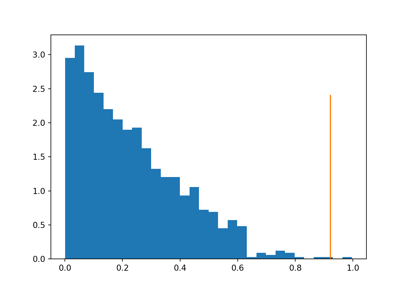

plt.plot((truediff, truediff), (0, 2.4))
plt.show()

Figure 4.1: Distribution of differences under non-stratified permutations, highlighting the observed true value.

plt.hist(meandiffs2, 30, density=True)

## (array([0.0237044 , 0.        , 0.0237044 , 0.0237044 , 0.09481758,
##        0.16593077, 0.26074835, 0.26074835, 0.40297473, 0.71113187,
##        0.66372308, 1.20892418, 1.25633297, 1.6356033 , 1.68301209,
##        2.32303078, 1.92005605, 2.08598682, 1.49337693, 1.58819451,
##        1.16151539, 1.49337693, 0.94817583, 0.73483627, 0.52149671,
##        0.16593077, 0.33186154, 0.30815714, 0.11852198, 0.09481758]), array([0.14980408, 0.19199034, 0.23417661, 0.27636288, 0.31854915,
##        0.36073542, 0.40292169, 0.44510796, 0.48729422, 0.52948049,
##        0.57166676, 0.61385303, 0.6560393 , 0.69822557, 0.74041183,
##        0.7825981 , 0.82478437, 0.86697064, 0.90915691, 0.95134318,
##        0.99352944, 1.03571571, 1.07790198, 1.12008825, 1.16227452,
##        1.20446079, 1.24664706, 1.28883332, 1.33101959, 1.37320586,
##        1.41539213]), <a list of 30 Patch objects>)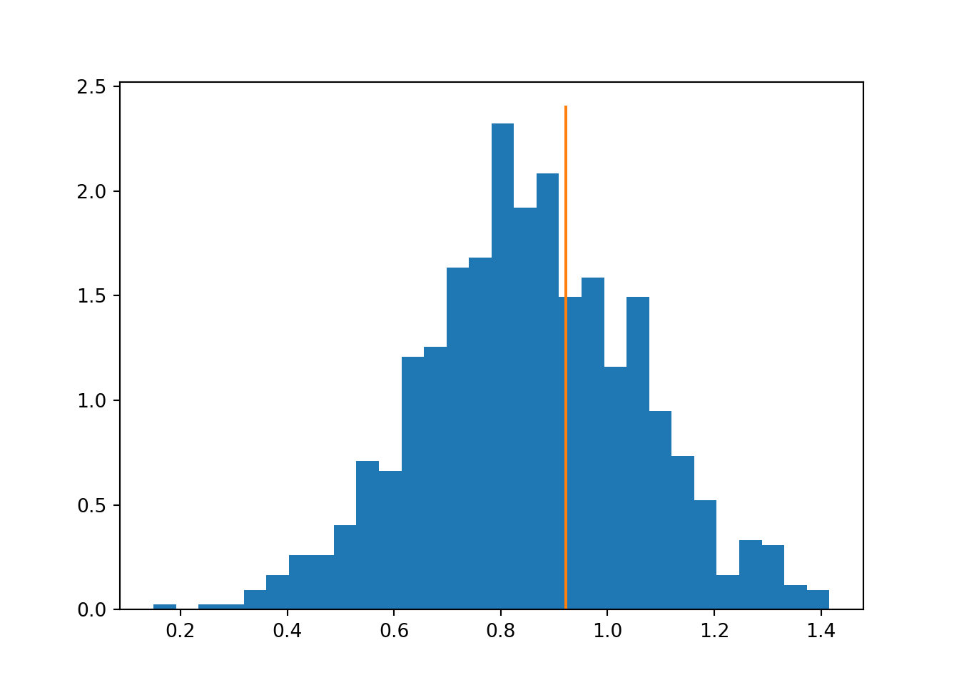

plt.plot((truediff, truediff), (0, 2.4))
plt.show()

Figure 4.2: Distribution of differences under stratified permutations, highlighting the observed true value.

4.2.2 Pros, cons and caveats of null-hypothesis significance testing

NHST can be a useful too for evaluating statistical significance, but it has a number of limitations:

\(p\)-values need to be interpreted with great care. Unlike commonly thought, \(p\)-value does not measure the probability that \(H_0\) is true.
\(p\)-values are only strictly valid for pre-specified tests. Any adaptivity in the analysis will destroy any theoretical guarantees.
Error control on the false positive probability of individual tests means that under multiple testing, the number of false positive errors can be very high. (5% probability of false positive in each test means on average 5 false positives from 100 tests. Multiple testing correction can help by setting more strict cutoffs here.)
Need to be careful about what is being tested: does “at least as extreme” consider one tail or two tails?

4.3 Bootstrap sampling

One of the fundamental questions of statistics is to translate results from an individual observed sample to the larger population. This involves the question of what could have happened, had the sample been drawn differently from the same larger population. More formally, especially frequentist statistics is interested in the performance of methods under repeated sampling from the data generating mechanism \(p(x)\).

Usually the true data generating mechanism \(p(x)\) is not known or accessible. Bootstrap sampling provides an accessible approach for computationally approximating computations requiring access to the data generating mechanism.

The Bootstrap principle suggests to approximate \(p(x)\) by sampling from the empirical data distribution \(p_e(x)\) with replacement. By sampling a data set of a given size, usually the same size as the original data set, we can estimate the uncertainty related to the sampling of the original data set.

The most common use of bootstrap sampling is the evaluation of confidence intervals for various statistical procedures, such as the estimation of some parameter \(\theta\).

Assuming the original data set \(X = (x_1, \dots, x_N)\) has \(N\) samples, bootstrap sampling works by generating \(M\) pseudo-data-sets \(X^*_i\), \(i = 1, \dots, M\), by always sampling \(N\) elements of \(X\) with replacement. Sampling with replacement implies that each pseudo-data-set is very likely to contain duplicates of some samples while missing others.

For each pseudo-data-set \(X^*_i\), ones obtains an estimate \(\theta^*_i\) of the parameter \(\theta\). Confidence intervals, such as the two-sided \(1-\alpha\) confidence interval can be obtained as \([h_{\alpha/2}, h_{1-\alpha/2}],\) where \(h_\alpha\) denotes the \(\alpha\) quantile of the bootstrap estimates \(\theta^*_i\).

More advanced bootstrap methods that may be more efficient are also available (Givens and Hoeting (2013)).

Example: confidence interval on the mean of a set of values

import numpy as np
import numpy.random as npr
 
npr.seed(42)
x = npr.normal(size=100)
 
print(np.mean(x))

## -0.10384651739409384

means = np.zeros(1000)
for i in range(1000):
    I = npr.randint(100, size=100)
    means[i] = np.mean(x[I])
print(np.percentile(means, [2.5, 97.5]))

## [-0.27233642  0.06285149]

4.4 Literature

Givens and Hoeting (2013) provide a good brief introduction to bootstrap. Permutation testing is nicely covered by Phipson and Smyth (2010), who also discuss the challenges with very small \(p\)-values.

References

Givens, Geof H., and Jennefer A. Hoeting. 2013. Computational Statistics. 2nd ed. Hoboken, NJ: Wiley.

Phipson, Belinda, and Gordon K Smyth. 2010. “Permutation P-Values Should Never Be Zero: Calculating Exact P-Values When Permutations Are Randomly Drawn.” Statistical Applications in Genetics and Molecular Biology 9: Article39. https://doi.org/10.2202/1544-6115.1585.