Chapter 13 Hamiltonian Monte Carlo (HMC)
Using gradient information of the target function can help improve MCMC convergence. Methods using this information are especially useful in high dimensions where a simple random walk has many more directions to wonder off and tracing a narrow high probability density shell will be very difficult.
13.1 Metropolis-adjusted Langevin algorithm
The simplest method for incorporating gradient information is the Metropolis-adjusted Langevin algorithm (MALA) (Roberts and Rosenthal (1998)) which simulates a reversible Langevin diffusion whose stationary distribution is the target \(\pi(\mathbf{\theta})\): \[ \mathrm{d}\mathbf{\theta}_t = \sigma \mathrm{d}B_t + \frac{\sigma^2}{2} \nabla \log \pi(\mathbf{\theta}_t) \mathrm{d}t. \] This expression is a stochastic differential equation, where \(B_t\) denotes the standard \(d\)-dimensional Brownian motion (a stochastic process with independent normally distributed increments).
Perhaps the simplest way to understand the Langevin diffusion is through its time discretisation: \[ \mathbf{\theta}'_{t+1} = \mathbf{\theta}_t + \sigma_n \mathbf{z}_{t+1} + \frac{\sigma_n^2}{2} \nabla \log \pi(\mathbf{\theta}_t), \] where \(\mathbf{z}_{t+1} \sim \mathcal{N}(0, \mathbf{I}_d).\)
With decreasing \(\sigma_n\), the discretisation gives better approximations of the original diffusion, but for a finite \(\sigma_n\), convergence to the correct stationary distribution will require the addition of the Metropolis-Hastings accept/reject step, where the proposal is accepted as usual with probability \[ \alpha(\mathbf{\theta}_t, \mathbf{\theta}'_{t+1}) = \frac{\pi(\mathbf{\theta}'_{t+1})}{\pi(\mathbf{\theta}_t)} \frac{q(\mathbf{\theta}_t; \mathbf{\theta}'_{t+1})}{q(\mathbf{\theta}'_{t+1}; \mathbf{\theta}_t)}, \] where \[ q(\mathbf{\theta}'_{t+1}; \mathbf{\theta}_t) = \mathcal{N}\left(\mathbf{\theta}'_{t+1};\; \mathbf{\theta}_t + \frac{\sigma_n^2}{2} \nabla \log \pi(\mathbf{\theta}_t), \sigma_n^2 \mathbf{I}_d \right). \]
MALA helps in finding a good direction which is important especially in high-dimensional spaces, but it still needs to take relatively short steps to achieve a high acceptance rate.
The MALA algorithm itself is not very widely used in practice, but recent work in machine learning has adopted it as a basis for stochastic gradient MCMC methods for MCMC with very large data sets.
13.2 Hamiltonian Monte Carlo (HMC)
Currently the most efficient general purpose samplers are based on Hamiltonian Monte Carlo (HMC). These can be developed through defining a dynamical system where \(- \log \pi(\mathbf{\theta})\) represents the potential energy of the system which is then simulated using Hamiltonian dynamics. Hamiltonian dynamics preserve the energy and volume of the system and by using a suitable (symplectic) numeric solver, the same applies even to the numerical solution. This allows simulating very long trajectories with a high acceptance probability.
For HMC we augment each regular “position” variable \(\mathbf{\theta}_i\) with a corresponding “momentum” variable \(\mathbf{r}_i \sim \mathcal{N}(0, 1)\) (denoted by \(\mathbf{p}_i\) in many of the more physical references). Denoting the potential energy defined by the target as \(U(\mathbf{\theta}) = -\log \pi(\mathbf{\theta})\), the momentum variables have a corresponding kinetic energy \(K(\mathbf{r}) = \sum_{i=1}^d \frac{1}{2} r_i^2\) with the total energy given by \(H(\mathbf{\theta}, \mathbf{r}) = U(\mathbf{\theta}) + K(\mathbf{r})\).
Hamiltonian dynamics of the system are defined by \[\begin{align*} \frac{\mathrm{d} \theta_i}{\mathrm{d}t} &= \frac{\partial H(\mathbf{\theta}, \mathbf{r})}{\partial r_i} \\ \frac{\mathrm{d} r_i}{\mathrm{d}t} &= - \frac{\partial H(\mathbf{\theta}, \mathbf{r})}{\partial \theta_i}. \end{align*}\]
For our choice of \(H(\mathbf{\theta}, \mathbf{r})\) these become \[\begin{align*} \frac{\mathrm{d} \theta_i}{\mathrm{d}t} &= r_i \\ \frac{\mathrm{d} r_i}{\mathrm{d}t} &= - \frac{\partial U(\mathbf{\theta})}{\partial \theta_i} = \frac{\partial \log \pi(\mathbf{\theta})}{\partial \theta_i}. \end{align*}\]
13.3 Numerical solution of Hamilton’s dynamics
The most common approach to simulate these equations numerically is to use the so-called leapfrog integrator which is specifically designed for Hamiltonian systems: \[\begin{align*} \mathbf{r}(t + \epsilon/2) &= \mathbf{r}(t) - (\epsilon/2) \nabla_{\mathbf{\theta}} U(\mathbf{\theta}(t)) \\ \mathbf{\theta}(t + \epsilon) &= \mathbf{\theta}(t) + \epsilon \mathbf{r}(t + \epsilon/2) \\ \mathbf{r}(t + \epsilon) &= \mathbf{r}(t + \epsilon/2) - (\epsilon/2) \nabla_{\mathbf{\theta}} U(\mathbf{\theta}(t + \epsilon)). \end{align*}\]
Compared to standard numerical differential equation solvers, the leapfrog integrator allows for stable solutions over a much longer time scale because the total energy of the system is conserved.
For more details, please see the excellent tutorial by Neal (2011).
Note: the HMC algorithm presented here can be extended to include “masses” for the “particles”, as suggested by Neal (2011). To simplify the notation we assume all “particles” have unit mass which may not be optimal for all applications.
13.4 HMC algorithm
The HMC algorithm is presented in pseudo-Python below.
The code assumes that target(theta) defines the target log-density
and gradF(theta) provides the gradients of the target.
Each step of the algorithm starts with simulating a normally distributed random momentum \(\mathbf{r}\). This is really a separate Metropolis-Hastings proposal, but because it is drawn from the exact conditional distribution of \(\mathbf{r}\), it will always be accepted.
Given this momentum, a trajectory of \(L\) leapfrog steps is simulated to obtain a new proposed pair \((\mathbf{\theta}', \mathbf{r}')\).
The proposed pair is then either accepted or rejected according to the Metropolis-Hastings acceptance rule in the augmented space of \((\mathbf{\theta}, \mathbf{r})\).
The logarithm of the acceptance probability \(\log a\) will depend on the difference of the total energies at the beginning and the end of proposed trajectories: \[ \log a = H(\mathbf{\theta}, \mathbf{r}) - H(\mathbf{\theta}', \mathbf{r}'), \] where \((\mathbf{\theta}, \mathbf{r})\) is the current state and \((\mathbf{\theta}', \mathbf{r}')\) is the proposed state obtained by simulating Hamilton’s dynamics for a number of steps. Because exact simulation preserves the energy, HMC with exact simulation would have acceptance probability \(a=1\) for all proposals, regardless of the length of the simulation. In practice the acceptance checks are still needed because of inexact simulation with a moderate \(\epsilon\).
g = gradF(theta)       # set gradient using initial theta
logP = target(theta)   # set log-target function too
for m in range(M): # collect M samples
    r ~ Normal(0, I)         # initial momentum is Normal(0,1)
    H = r.T @ r / 2 - logP   # evaluate H(theta,r)
    thetanew = theta
    gnew = g
    for l in range(L):       # make L 'leapfrog' steps
        r = r + epsilon * gnew / 2   # make half-step in r
        thetanew = thetanew + epsilon * r    # make step in theta
        gnew = gradF(thetanew)           # find new gradient
        r = r + epsilon * gnew / 2   # make half-step in r
    logPnew = target(thetanew)           # find new value of H
    # in theory we should now set r = -r to make the chain reversible,
    # but as we are not storing r values this makes no difference
    Hnew = r.T @ r / 2 - logPnew
    dH = Hnew - H    # Decide whether to accept
    if np.log(npr.rand()) < -dH:
        g = gnew
        theta = thetanew
        logP = logPnew
13.5 Tuning HMC
HMC has two tunable parameters: \(\epsilon\) and \(L\).
Out of these, \(\epsilon\) is usually easier to tune, because it affects the accuracy of the numerical integration and thus the acceptance rate. Unlike the gradual change in acceptance probability when tuning random walk MCMC proposals, the effect of increasing \(\epsilon\) can be quite dramatic. At first, the acceptance rate is very close to 1 but at some point after a steep decline it drops to 0.
Because of the heavier computation in computing the proposal, the optimal acceptance rate for HMC is higher than for random walk MCMC. Acceptance rate of approximately 0.8 is in general a good target. \(\epsilon\) values of the order 0.1 seem to work well for many problems, but obviously this can be problem-dependent.
Tuning \(L\) is more difficult. HMC leapfrog trajectories can resemble the flight path of a boomerang that starts moving away but at some point will turn back to the starting point. At \(L=1\) HMC reduces to random walk MCMC, so larger \(L\) are needed to benefit from the more complicated algorithm. At the same time, too large \(L\) can at worst lead to very inefficient sampling when the trajectories will return back to their starting point.
In general, the optimal \(L\) will vary by trajectory. This challenge is addressed by dynamic HMC algorithms such as the No-U-Turn Sampler (NUTS) introduced in Chapter 14.
13.6 HMC theory
Ultimately, the HMC sampler introduced above is just a Metropolis-Hastings sampler with a very complex proposal. Because of this, the Metropolis-Hastings acceptance check guarantees detailed balance and convergence to the desired distribution.
The HMC proposal yields an ergodic chain, except if integration paths are periodic (this can happen e.g. when the target is normal) and the path length matches the period length. This can be avoided by randomising path or step lengths at different iterations, e.g. \(\epsilon = v \epsilon_0\) with \(v \sim \mathrm{Uniform}(0.8, 1.2)\).
Finally, while HMC provides extremely efficient sampling for unimodal distributions, it does not solve the problem of multiple modes. In a multimodal distribution, HMC can in theory jump across modes, but only if it happens to sample a sufficiently large momentum \(\mathbf{r}\) in exactly the right direction, which can be very rare if the modes are well-separated. Other techniques like parallel tempering are still required to address the issue properly, possibly in combination with HMC.
13.7 Examples
As an example, we illustrate HMC sampling on a spherical density \[ \log \pi(\mathbf{\theta}) = -20 (\|\mathbf{\theta}\|_2 - 10)^2, \] which in 2D reduces to a circle.
This is a difficult target for random walk MCMC that can only move slowly around the circle. HMC with sufficiently large \(L\) on the other hand can jump across the circle in one move with very high acceptance probability, as illustrated by the below line plots connecting consecutive points. Here already 100 samples without any thinning are sufficient for a reasonable coverage around the circle.
import autograd.numpy as np
import autograd.numpy.random as npr
import autograd
import matplotlib.pyplot as plt

def hmc(theta0, M, target, epsilon, L):
    thetas = np.zeros([M, len(theta0)])
    gradF = autograd.grad(target)
    theta = np.copy(theta0)
    g = gradF(theta)  # set gradient using initial theta
    logP = target(theta)  # set objective function too
    accepts = 0
    for m in range(M): # draw M samples
        p = npr.normal(size=theta.shape)  # initial momentum is Normal(0,1)
        H = p.T @ p / 2 - logP   # evaluate H(theta,p)
        thetanew = np.copy(theta)
        gnew = np.copy(g)
        for l in range(L): # make L 'leapfrog' steps
            p = p + epsilon * gnew / 2   # make half-step in p
            thetanew = thetanew + epsilon * p    # make step in theta
            gnew = gradF(thetanew)           # find new gradient
            p = p + epsilon * gnew / 2   # make half-step in p
        logPnew = target(thetanew)   # find new value of H
        Hnew = p.T @ p / 2 - logPnew
        dH = H - Hnew    # Decide whether to accept
        if np.log(npr.rand()) < dH:
            g = gnew
            theta = thetanew
            logP = logPnew
            accepts += 1
        thetas[m,:] = theta
    print('Acceptance rate:', accepts/M)
    return thetas

def sphere(theta):
    return -20*(np.sqrt(np.sum(theta**2))-10)**2

samples = hmc(np.array([3.0, 0.0]), 200, lambda theta: sphere(theta), 0.2, 50)
## Acceptance rate: 0.9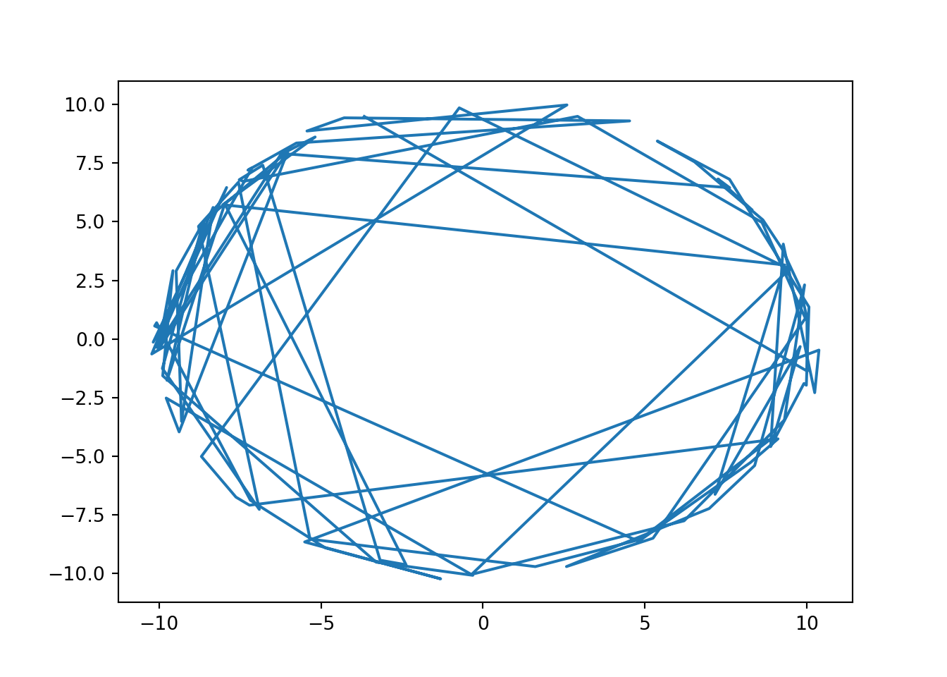
import torch
import matplotlib.pyplot as plt

torch.set_default_dtype(torch.double)
# Uncomment this to run on GPU
# torch.set_default_tensor_type(torch.cuda.DoubleTensor)

def sphere(theta):
    return -20*(torch.sqrt(torch.sum(theta**2))-10)**2

def hmc(theta0, M, target, epsilon, L):
    thetas = torch.zeros([M, len(theta0)])
    theta = theta0.clone().detach().requires_grad_(True)
    logP = target(theta)  # set objective function too
    logP.backward()
    g = theta.grad
    accepts = 0
    for m in range(M): # draw M samples
        p = torch.normal(torch.zeros(theta.shape))  # initial momentum is Normal(0,1)
        H = p.dot(p) / 2 - logP   # evaluate H(theta,p)
        thetanew = theta.clone().detach().requires_grad_(True)
        gnew = g.clone().detach()
        for l in range(L): # make L 'leapfrog' steps
            p.data += epsilon * gnew.data / 2   # make half-step in p
            thetanew.data += epsilon * p.data          # make step in theta
            if thetanew.grad is not None:
                thetanew.grad.zero_()
            logPnew = target(thetanew)
            logPnew.backward()
            gnew = thetanew.grad             # find new gradient
            p.data += epsilon * gnew.data / 2   # make half-step in p
        logPnew = target(thetanew)   # find new value of H
        Hnew = p.dot(p) / 2 - logPnew
        dH = H - Hnew    # Decide whether to accept
        if torch.log(torch.rand(1)) < dH:
            g = gnew
            theta = thetanew
            logP = logPnew
            accepts += 1
        thetas[m,:] = theta.detach()
    print('Acceptance rate:', accepts/M)
    return thetas

# Set the seed for PyTorch RNGs
torch.manual_seed(42)
## <torch._C.Generator object at 0x7fa887999af0>## Acceptance rate: 0.875samples = samples[samples.shape[0]//2:]
plt.plot(samples.numpy()[:,0], samples.numpy()[:,1])
plt.show()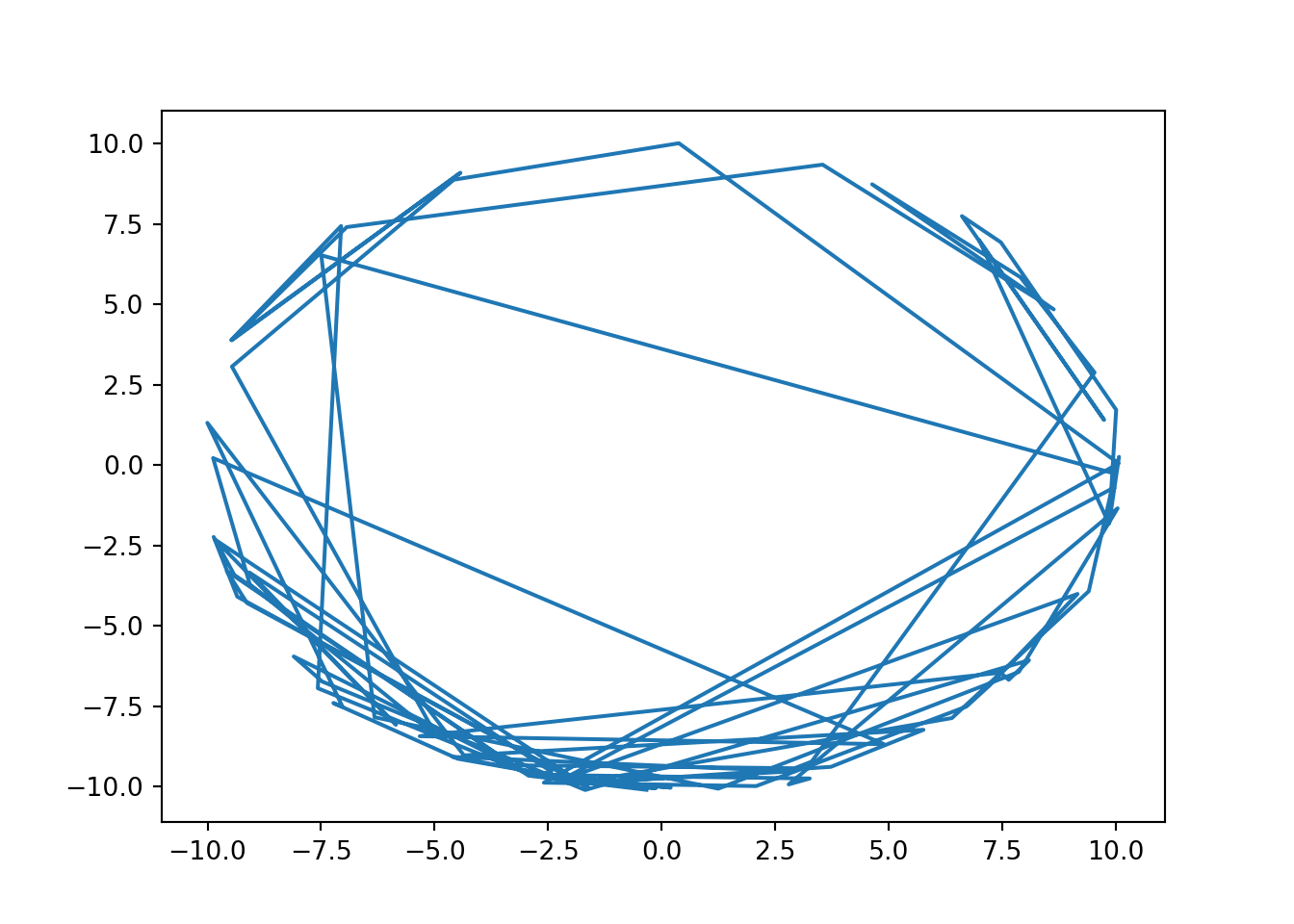
References
Betancourt, Michael. 2017. “A Conceptual Introduction to Hamiltonian Monte Carlo,” January. http://arxiv.org/abs/1701.02434.
Neal, Radford M. 2011. “MCMC Using Hamiltonian Dynamics.” In Handbook of Markov Chain Monte Carlo, edited by Steve Brooks, Andrew Gelman, Galin Jones, and Xiao-Li Meng. Chapman & Hall/CRC. http://arxiv.org/abs/1206.1901.
Roberts, Gareth O., and Jeffrey S. Rosenthal. 1998. “Optimal Scaling of Discrete Approximations to Langevin Diffusions.” Journal of the Royal Statistical Society: Series B (Statistical Methodology) 60 (1): 255–68. https://doi.org/10.1111/1467-9868.00123.