Chapter 6 Markov chain Monte Carlo basics
The simple methods introduced in Chapter 2 for simulating pseudorandom numbers are insufficient for simulating complicated distributions.
This need is especially clear when one needs to draw samples from the posterior distribution of a Bayesian probabilistic model (more details in Chapter 7), because the posterior distribution often depends on an intractable normalising factor.
Markov chain Monte Carlo (MCMC) methods are based on a simple idea: instead of sampling the target distribution directly, the goal is to develop a Markov chain that converges to the correct distribution.
6.1 Markov chains
The possible values of all \(\theta_t\) variables are called the states of the chain. The space of possible states can be finite, countably infinite or even continuous.
The definition implies that a Markov chain effectively has no memory: all knowledge of the past that affects the future is contained in the current state.
Because of the Markov property, a Markov chain is fully defined by the initial distribution \(p(\theta_1)\) and the transition kernel \(T(\theta_{t-1}, \theta_t) = p(\theta_t | \theta_{t-1})\).
6.2 Markov chain convergence theory
For MCMC we will need to focus on Markov chains that converge to a stationary distribution, which needs to be the desired target distribution.
Below are some important concepts for Markov chains related to the convergence.
The lack of irreducibility means that there are two or more classes of states for which the chain cannot move between the classes. This obviously prevents the chain from converging in general.
Ergodicity is an important property for Markov chains as it guarantees that the chain is in essence well-behaved and can move around the state space without obstructions.
A reversible Markov chain is always stationary.
A Markov chain that satisfies the detailed balance is reversible.
Finally, every reversible ergodic Markov chain has a unique stationary distribution.
6.3 Metropolis-Hastings algorithm
Metropolis-Hastings (MH) sampling works by deriving a Markov chain \(\theta^{(1)}, \theta^{(2)}, \dots\) whose stationary distribution is the target \(\pi(\theta)\). The algorithm works by proposing a new state \(\theta'\) from a proposal density \(q(\theta' ; \theta^{(t)})\). The proposal is either accepted or rejected based on the quantity \[\begin{equation} a = \frac{\pi(\theta')}{\pi(\theta^{(t)})} \frac{q(\theta^{(t)} ; \theta')}{q(\theta' ; \theta^{(t)})} \tag{6.1} \end{equation}\] as follows:
- If \(a \ge 1\), then the new state is always accepted.
- Otherwise, the new state is accepted with probability \(a\).
If the step is accepted, we set \(\theta^{(t+1)} = \theta'\).
If the step is rejected, then we set \(\theta^{(t+1)} = \theta^{(t)}\).
The MH update fulfils detailed balance and the chain is thus reversible. The chain is also ergodic if the proposal is chosen suitably. A sufficient condition for ergodicity is that there exists a finite \(n_0\) such that any state can be reached from any other state in \(n\) steps for all \(n \ge n_0\).
There is an important special case of the MH algorithm when the proposal \(q\) is symmetric: \(q(\theta^{(t)} ; \theta') = q(\theta' ; \theta^{(t)})\). This happens for example when the proposal follows a fixed symmetric distribution centred around the current value, such as \[ q(\theta' ; \theta) = \mathcal{N}(\theta';\; \theta, \sigma^2). \] In this case the acceptance probability will simplify to \[ a = \frac{\pi(\theta')}{\pi(\theta^{(t)})}. \] This special case is often referred to as the Metropolis algorithm.
Note that MH-sampling only requires the ratio of the target probability densities \(\frac{\pi(\theta')}{\pi(\theta^{(t)})}\). This implies that we can use an unnormalised density \(\pi^*(\theta) = Z \cdot \pi(\theta)\) with unknown but fixed normaliser \(Z\) and obtain the same results.
We will now illustrate this with an example drawing samples from the Laplace distribution \(\pi^*(\theta) = \exp(-|\theta|)\) using the normal proposal \(q(\theta' ; \theta) = \mathcal{N}(\theta';\; \theta, \sigma^2)\) centred around the current value using \(\sigma^2=1\).
6.3.1 Implementation of the Metropolis-Hastings algorithm
To implement the MH algorithm in software, it is always better to use log-densities instead of the raw density values for numerical stability.
Taking logs of the acceptance probability yields \[ \log a = \log \pi(\theta') - \log \pi(\theta^{(t)}) + \log q(\theta^{(t)} ; \theta') - \log q(\theta' ; \theta^{(t)}), \] or in the symmetric-\(q\) plain Metropolis case \[ \log a = \log \pi(\theta') - \log \pi(\theta^{(t)}). \]
The acceptance rule contains a condition to accept a proposal with probability \(a\). This can be implemented by sampling a random number \(u \sim \mathrm{Uniform}(0, 1)\), and checking if \(u < a\), which will happen with probability \(a\).
The acceptance rule tells to always accept if \(a > 1\). This does not need to be checked separately because \[ a > 1 \Rightarrow u < a. \]
Finally, because \(\log\) is a monotone increasing function, we can take the log of the acceptance check to arrive at a rule to accept if \[ \log u < \log \pi(\theta') - \log \pi(\theta^{(t)}) + \log q(\theta^{(t)} ; \theta') - \log q(\theta' ; \theta^{(t)}), \] where \(u \sim \mathrm{Uniform}(0, 1)\).
If we know \(q\) is symmetric, we know \(\log q(\theta^{(t)} ; \theta') - \log q(\theta' ; \theta^{(t)}) = 0,\) and thus we can avoid computing \(q\) for example by setting it to some constant value in the code.
MCMC depends on the initial state. In order to remove the dependence of the samples from the initial state, it is common to discard the first half of the samples as warm-up samples.
In the example below, we make use of the lambda construct
to construct new functions to pass as argument to define the target and the proposal. This construct is very useful because it allows to easily create a new function using existing functions with some arguments fixed.
import numpy as np
import numpy.random as npr
import matplotlib.pyplot as plt

# Metropolis sampling (symmetric proposal) for given log-target distribution
def mhsample0(theta0, n, logtarget, drawproposal):
    theta = theta0
    thetas = np.zeros(n)
    for i in range(n):
        theta_prop = drawproposal(theta)
        if np.log(npr.rand()) < logtarget(theta_prop) - logtarget(theta):
            theta = theta_prop
        thetas[i] = theta
    return thetas

# Testing Laplace target with normal proposal centred around the previous value
npr.seed(42)
theta = mhsample0(0.0, 10000, lambda theta: -np.abs(theta),
                  lambda theta: theta+npr.normal())

# Discard the first half of samples as warm-up
theta = theta[len(theta)//2:]
fig, ax = plt.subplots(1, 2)
ax[0].plot(theta[::10])
h = ax[1].hist(theta[::10], 50, density=True)
plt.show()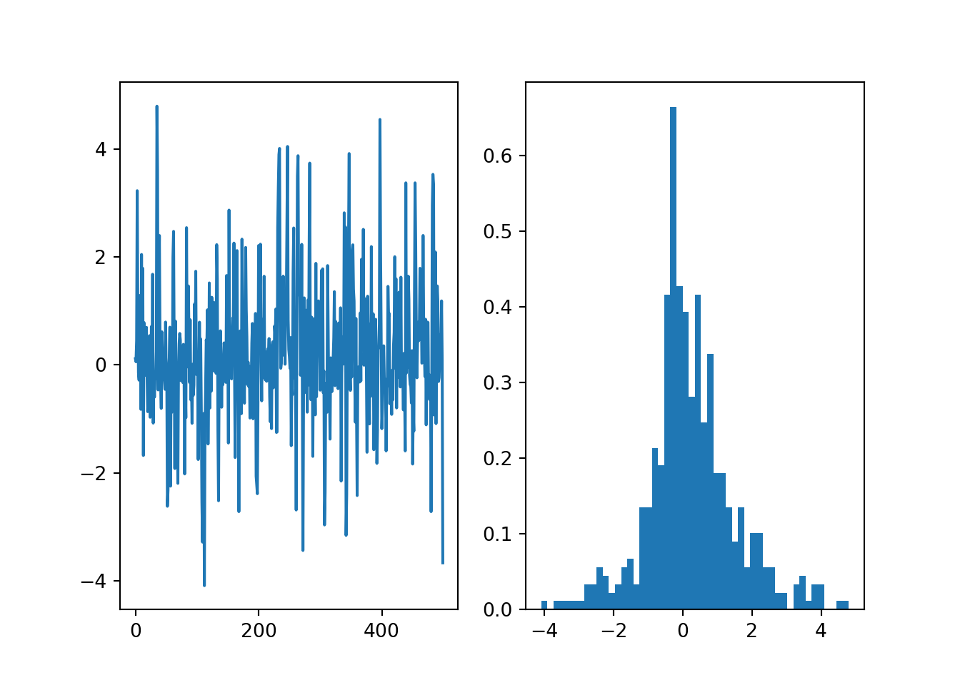
6.4 MCMC sampling efficiency
The efficiency of an MCMC sampler depends on the proposal \(q(\theta' ; \theta)\). We can test this in the setting of the above example by changing the value of \(\sigma^2\) while augmenting the function to compute the fraction of accepted steps.
# Metropolis sampling (symmetric proposal) for given log-target distribution
def mhsample1(theta0, n, logtarget, drawproposal):
    theta = theta0
    thetas = np.zeros(n)
    accepts = 0
    for i in range(n):
        theta_prop = drawproposal(theta)
        if np.log(npr.rand()) < logtarget(theta_prop) - logtarget(theta):
            theta = theta_prop
            accepts += 1
        thetas[i] = theta
    print("Sampler acceptance rate:", accepts/n)
    return thetas

# Testing Laplace target with a narrow normal proposal
theta = mhsample1(0.0, 10000, lambda theta: -np.abs(theta),
                  lambda theta: theta+0.1*npr.normal())

# Discard the first half of samples as warm-up
## Sampler acceptance rate: 0.9612theta = theta[len(theta)//2:]
fig, ax = plt.subplots(1, 2)
ax[0].plot(theta[::10])
h = ax[1].hist(theta[::10], 50, density=True)
plt.show()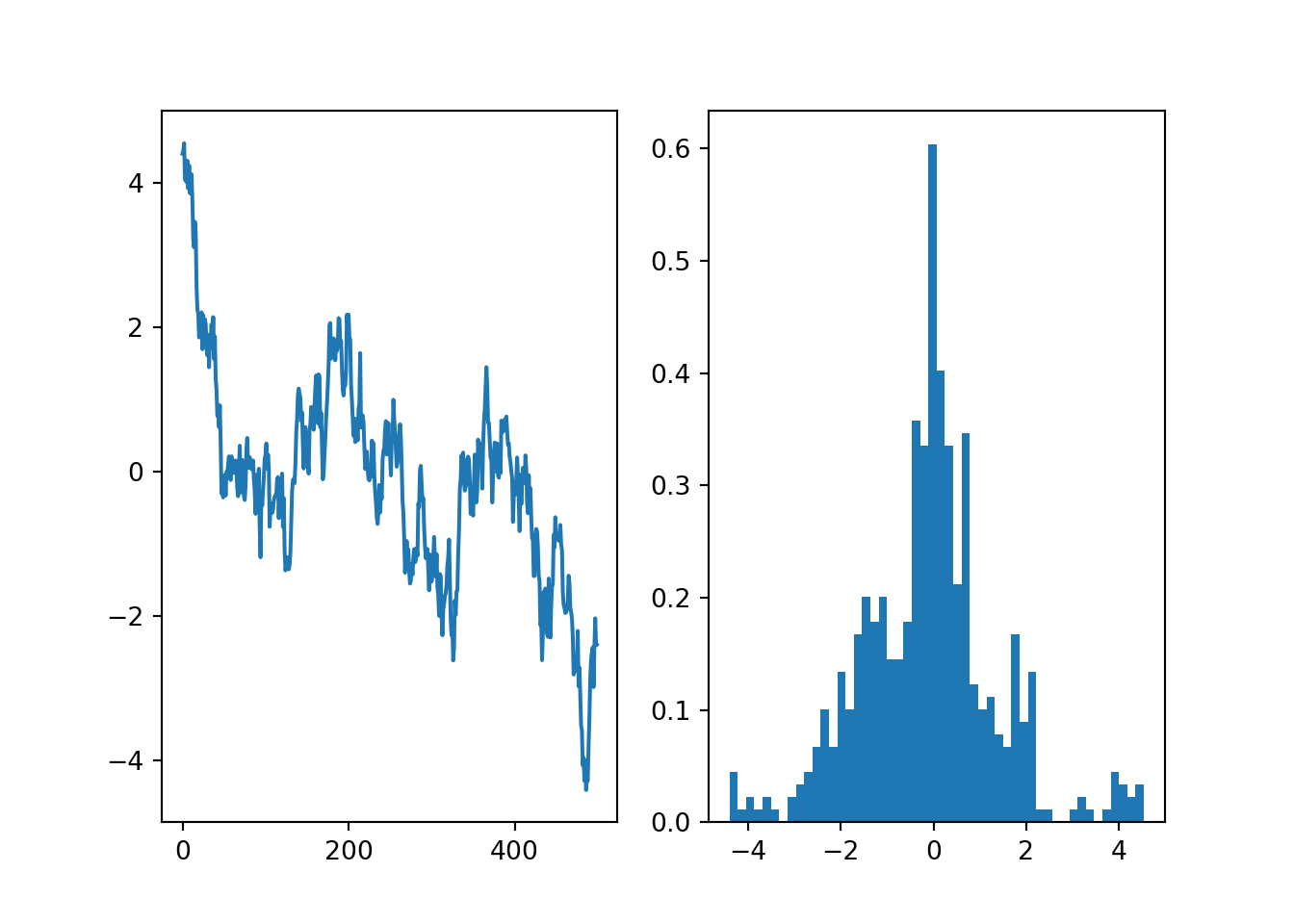
# Testing Laplace target with a well-tuned normal proposal
theta = mhsample1(0.0, 10000, lambda theta: -np.abs(theta),
                  lambda theta: theta+2.5*npr.normal())

# Discard the first half of samples as warm-up
## Sampler acceptance rate: 0.4642theta = theta[len(theta)//2:]
fig, ax = plt.subplots(1, 2)
ax[0].plot(theta[::10])
h = ax[1].hist(theta[::10], 50, density=True)
plt.show()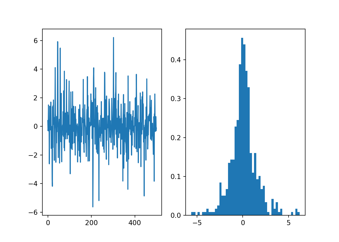
# Testing Laplace target with a wide normal proposal
theta = mhsample1(0.0, 10000, lambda theta: -np.abs(theta),
                  lambda theta: theta+50*npr.normal())

# Discard the first half of samples as warm-up
## Sampler acceptance rate: 0.0345theta = theta[len(theta)//2:]
fig, ax = plt.subplots(1, 2)
ax[0].plot(theta[::10])
h = ax[1].hist(theta[::10], 50, density=True)
plt.show()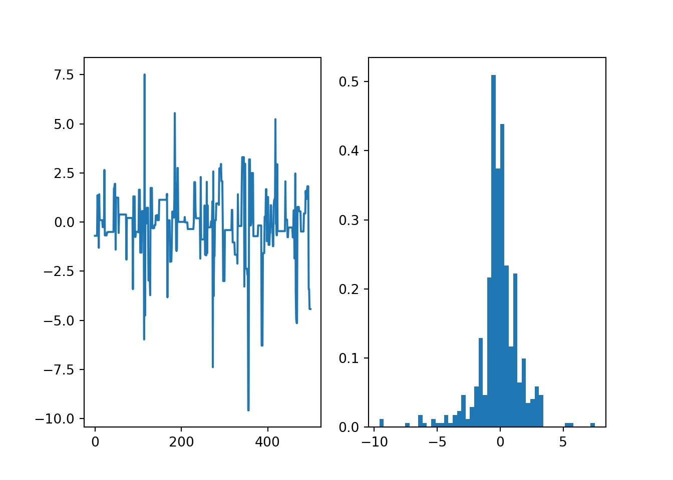
We can see that too narrow proposals lead to very high acceptance rates but persistent random walks that can seriously bias the sample. Too wide proposals lead to very low acceptance rates and long sequences of identical states that can be seen as spikes in the histogram of the samples. These will eventually all be smoothed out as the sampler will converge to the correct target distribution, but if the proposal is poorly chosen, this can take an impractically long time.
The proposal is usually tuned with a scalar parameter that determines the step length, monitoring the acceptance rate. The optimal acceptance rate for Metropolis-Hastings for unimodal targets is quite low: ranging from 50% (low dimensional) down to 23% (high dimensional). These have been derived for sampling a multivariate normal distribution target, but can be expected to generalise to other unimodal distributions. High acceptance usually indicates too short steps, low acceptance indicates too long steps.
A good practice for MH is to tune the proposal width until the acceptance rate is in this range.
It should be stressed that the above optimal acceptance does not apply in general to multimodal targets, i.e. distributions that have several separate modes of high probability. Sampling such distributions with MCMC is difficult at best, and usually the most important determinant of the accuracy is how well the sampler can jump between the modes which can be poorly captured by the standard acceptance rate.
6.5 Convergence of the Metropolis-Hastings algorithm
Let us assume that the proposal is such that any state \(\theta'\) with \(\pi(\theta') > 0\) can be reached from any other state in \(n\) steps for all \(n \ge n_0\) for some \(n_0\).
This guarantees that the Markov chain defined by the MH algorithm is ergodic. Together with the following theorem showing that the chain satisfies the detailed balance condition, these guarantee that the chain will converge to produce samples from the target distribution \(\pi(\theta)\).
From the perspective of the above theory, it is sufficient that the proposal allows arbitrary transitions after a number of steps. This is usually satisfied by typical proposal distributions such as normal distribution, although finite precision arithmetic may cause trouble in some extreme cases with strongly separated modes.
6.5.1 Notes on MCMC convergence
The above theory shows that when the proposal is OK, the Markov chain defined by the MH algorithm will eventually converge to produce samples from the target distribution. It is important to note that this is an asymptotic guarantee - it is very hard or impossible to make any claims about convergence after any finite number of steps.
While essentially any reasonable proposal is enough to guarantee asymptotic convergence, the convergence speeds depends strongly on the specific proposal used. This is why it is important to tune the proposal for the problem at hand.
The MCMC convergence theory assumes that the transition kernel does not depend on past samples. Tuning the proposal or even adaptive termination criteria can break these assumptions. There are adaptive samplers that can avoid these issues, but they are more complicated and not very widely used. Ignoring all samples from the tuning/tweaking phase is usually the best choice.
It is in general impossible to prove a Markov chain has converged - you can never tell if you are just stuck exploring a local mode.
When run for a finite time, MCMC is in general a method for approximate inference even though some people claim it is exact.
6.5.2 Convergence of Monte Carlo expectations
Sampling expectations converge almost surely to corresponding expectations under the stationary distribution \[ \lim\limits_{N \rightarrow \infty} \frac{1}{N} \sum_{i=1}^N h(\theta_i) \rightarrow \operatorname{E}_\pi[h(\theta)] = \int h(\theta) \pi(\theta) \,\mathrm{d} \theta, \] assuming \(\int |h(\theta)| \pi(\theta) \,\mathrm{d} \theta < \infty.\)
The speed of convergence is determined by a central limit theorem \[ \sqrt{N} \left( \frac{1}{N} \sum_{i=1}^N h(\theta_i) - \operatorname{E}_\pi[h(\theta)] \right) \overset{d}{\rightarrow} \mathcal{N}(0, \sigma_h^2). \]
This implies a convergence rate of \(\mathcal{O}(1/\sqrt{n})\), which means that in order to double the accuracy, the number of samples must be increased by a factor of 4.
6.6 Initial best practices (to be completed later)
- Samples from an initial warm-up or burn-in period (e.g. first 50% of samples) are discarded as they depend too much on the initial point.
- The proposal often needs to be tuned to get fast mixing. You should first perform any tuning, then discard all those samples and run the actual analysis. Note that the optimal tuning for warm-up and stationary phases might be different.
Gelman and Shirley (2011)
6.7 Literature
Koistinen (2013) provides a nice introduction to MCMC theory for the more mathematically inclined readers.
References
Gelman, Andrew, and Kenneth Shirley. 2011. “Inference and Monitoring Convergence.” In Handbook of Markov Chain Monte Carlo, edited by Steve Brooks, Andrew Gelman, Galin Jones, and Xiao-Li Meng. Chapman & Hall/CRC. http://www.mcmchandbook.net/HandbookChapter6.pdf.
Koistinen, Petri. 2013. “Computational Statistics.”