Chapter 7 Bayesian inference with MCMC
The most important use for MCMC sampling in statistics is in Bayesian inference and drawing samples from the posterior distribution of a probabilistic model.
7.1 Bayesian inference
Given the observations \(\mathcal{D}\), a model \(p(\mathcal{D} | \theta)\) with parameters \(\theta\), and prior probability \(p(\theta)\) of the parameters, the posterior probability distribution of the parameters, i.e. the distribution of the parameters given the data, is given by the Bayes’ rule \[\begin{equation} p(\theta | \mathcal{D}) = \frac{p(\mathcal{D} | \theta) p(\theta)}{p(\mathcal{D})} = \frac{p(\mathcal{D} | \theta) p(\theta)}{\int_{\theta} p(\mathcal{D} | \theta) p(\theta) \;\mathrm{d}\theta}. \tag{7.1} \end{equation}\] While \(p(\mathcal{D} | \theta)\) and \(p(\theta)\) are usually known and easy to handle, this expression cannot usually be used directly because of the integral in the denominator \[ p(\mathcal{D}) = \int_{\theta} p(\mathcal{D} | \theta) p(\theta) \,\mathrm{d} \theta, \] whose result is known as the marginal likelihood or the evidence. This quantity is important for higher level inference over different models, but in terms of the posterior distribution it is just a scalar normaliser.
Example 7.1 Let us consider Bayesian inference of the mean \(\mu\) of normally distributed data \(\mathcal{D} = (x_1, \dots, x_n)\) with known variance \(\sigma_x^2\).
Assuming the observations are independent given \(\mu\), the model depending on the parameter \(\theta = \{ \mu \}\) is \[ p(\mathcal{D} | \theta) = \prod_{i=1}^n p(x_i | \mu) = \prod_{i=1}^n \mathcal{N}(x_i ;\; \mu, \sigma_x^2). \]
In order to perform Bayesian inference on the model, we need a prior \(p(\theta) = p(\mu)\) for the unknown parameter. The prior should reflect our beliefs about the value of the parameter. Prior choice is an important question in Bayesian modelling, but we will not discuss it further during this course. (See e.g. Gelman et al. (2013) for a detailed discussion.) For this example, we use a normal prior \[ p(\mu) = \mathcal{N}(\mu ;\; \mu_0, \sigma_0^2) \] with some specified \(\mu_0, \sigma_0^2\), which is a very common choice in this situation.
In this case the prior has a specific form which allows exact derivation of the posterior as \[ p(\mu | \mathcal{D}) \propto p(\mathcal{D} | \mu) p(\mu) = \prod_{i=1}^n \mathcal{N}(x_i ;\; \mu, \sigma_x^2) \mathcal{N}(\mu ;\; \mu_0, \sigma_0^2).\] Taking logs and ignoring all additive constants, this can be simplified to \[\begin{align*} \log p(\mu | \mathcal{D}) &= \sum_{i=1}^n - \frac{(x_i - \mu)^2}{2 \sigma_x^2} - \frac{(\mu - \mu_0)^2}{2 \sigma_0^2} + C \\ &= - \frac{n \left( \frac{1}{n}\sum_{i=1}^n x_i - \mu\right)^2}{2 \sigma_x^2} - \frac{(\mu - \mu_0)^2}{2 \sigma_0^2} + C'. \end{align*}\] Denoting \(\bar{x} = \frac{1}{n}\sum_{i=1}^n x_i\), we obtain \[\begin{align*} \log p(\mu | \mathcal{D}) &= - \frac{n ( \bar{x} - \mu)^2}{2 \sigma_x^2} - \frac{(\mu - \mu_0)^2}{2 \sigma_0^2} + C' \\ &= - \frac{n \sigma_0^2 ( \bar{x} - \mu)^2 + \sigma_x^2 (\mu - \mu_0)^2}{2 \sigma_x^2 \sigma_0^2} + C' \\ &= - \frac{n \sigma_0^2 (\bar{x}^2 - 2 \bar{x} \mu + \mu^2) + \sigma_x^2 (\mu^2 - 2 \mu \mu_0 + \mu_0^2)}{2 \sigma_x^2 \sigma_0^2} + C' \\ &= - \frac{(n \sigma_0^2 + \sigma_x^2) \mu^2 - 2 (n \sigma_0^2 \bar{x} + \sigma_x^2 \mu_0) \mu + n \sigma_0^2 \bar{x}^2 + \sigma_x^2 \mu_0^2)}{2 \sigma_x^2 \sigma_0^2} + C' \\ &= - (n \sigma_0^2 + \sigma_x^2) \frac{\mu^2 - 2 \frac{n \sigma_0^2 \bar{x} + \sigma_x^2 \mu_0}{n \sigma_0^2 + \sigma_x^2} \mu + \frac{n \sigma_0^2 \bar{x}^2 + \sigma_x^2 \mu_0^2}{n \sigma_0^2 + \sigma_x^2}}{2 \sigma_x^2 \sigma_0^2} + C' \\ &= -(n \sigma_0^2 + \sigma_x^2) \frac{[\mu^2 - \frac{n \sigma_0^2 \bar{x} + \sigma_x^2 \mu_0}{n \sigma_0^2 + \sigma_x^2}]^2}{2 \sigma_x^2 \sigma_0^2} + C'' \end{align*}\] The last form can be recognised as the log-density of the normal distribution \(\mathcal{N}(\mu;\; \mu_{\mu}^*, \sigma_{\mu}^{2^*})\) with \[\begin{align*} \mu_{\mu}^* &= \frac{n \sigma_0^2 \bar{x} + \sigma_x^2 \mu_0}{n \sigma_0^2 + \sigma_x^2} \\ \sigma_{\mu}^{2^*} &= \frac{\sigma_x^2 \sigma_0^2}{n \sigma_0^2 + \sigma_x^2} = \left( \frac{n}{\sigma_x^2} + \frac{1}{\sigma_0^2} \right)^{-1}. \end{align*}\]The model used here is special because the prior used is conjugate to the likelihood, which implies that the posterior will have the same functional form as the prior. However as seen above, even in this very simple case, deriving the posterior required quite tedious derivations.
7.2 Sampling the posterior with MCMC
As demonstrated by Example 7.1, the numerator of Eq. (7.1) is often easy to compute while the scalar normaliser \(p(\mathcal{D})\) usually is not. This makes posterior sampling an excellent application for MCMC because the Metropolis-Hastings algorithm can work with an unnormalised density.
Given a data set, we can apply the Metropolis-Hastings algorithm defined in Sec. 6.3 to Example 7.1 by defining the target as: \[ \log \pi^*(\theta) = \log p(\mathcal{D} | \mu) + \log p(\mu) = \sum_{i=1}^n \log \mathcal{N}(x_i ;\; \mu, \sigma_x^2) + \log \mathcal{N}(\mu ;\; \mu_0, \sigma_0^2). \]
We will fix the parameters at \(\sigma_x^2 = 1, \mu_0 = 0, \sigma_0^2 = 3^2\).
Using a normal proposal \(q(\theta' ; \theta) = \mathcal{N}(\theta';\; \theta, \sigma_{\text{prop}}^2),\) we can implement this as follows. The resulting samples and the corresponding analytical posterior are compared in Fig. 7.1.
# Define the normal pdf. Note parameters: mean, standard deviation
# Note the sum to allow evaluation for a data set at once
def lnormpdf(x, mu, sigma):
    return np.sum(-0.5*np.log(2*np.pi) - np.log(sigma) - 0.5 * (x-mu)**2/sigma**2)

# Define the target log-pdf as a sum of likelihood and prior terms
def target(mu, data, sigma_x, mu0, sigma0):
    return lnormpdf(data, mu, sigma_x) + lnormpdf(mu, mu0, sigma0)

# Simulate n=100 points of normally distributed data about mu=0.5
n = 100
data = 0.5 + npr.normal(size=n)

# Set the prior parameters
sigma_x = 1.0
mu0 = 0.0
sigma0 = 3.0

# Run the sampler
theta = mhsample1(0.0, 10000,
                  lambda mu: target(mu, data, sigma_x, mu0, sigma0),
                  lambda theta: theta+0.2*npr.normal())

# Discard the first half of samples as warm-up
## Sampler acceptance rate: 0.4975theta = theta[len(theta)//2:]
# Plot a histogram of the posterior samples
plt.hist(theta, 30, density=True)
# Compare with analytical result from the above example## (array([0.05091727, 0.16972423, 0.23761392, 0.77224526, 0.86559358,
## 1.06077645, 1.70572853, 2.06214942, 2.97866027, 3.59815372,
## 3.50480539, 3.81879522, 5.04080969, 3.60663993, 3.25870525,
## 2.30824956, 1.96031488, 1.65481126, 1.32384901, 0.84013495,
## 0.51765891, 0.43279679, 0.3649071 , 0.11880696, 0.04243106,
## 0.08486212, 0.00848621, 0. , 0.02545863, 0.01697242]), array([0.09811182, 0.12167946, 0.14524711, 0.16881475, 0.19238239,
## 0.21595003, 0.23951767, 0.26308532, 0.28665296, 0.3102206 ,
## 0.33378824, 0.35735589, 0.38092353, 0.40449117, 0.42805881,
## 0.45162646, 0.4751941 , 0.49876174, 0.52232938, 0.54589703,
## 0.56946467, 0.59303231, 0.61659995, 0.64016759, 0.66373524,
## 0.68730288, 0.71087052, 0.73443816, 0.75800581, 0.78157345,
## 0.80514109]), <a list of 30 Patch objects>)tt = np.linspace(0.1, 0.9, 50)
m_post = sigma0**2 * np.sum(data) / (n*sigma0**2 + sigma_x**2)
s2_post = 1/(n/sigma_x**2 + 1/sigma0**2)
y = np.array([np.exp(lnormpdf(t, m_post, np.sqrt(s2_post))) for t in tt])
plt.plot(tt, y)
plt.show()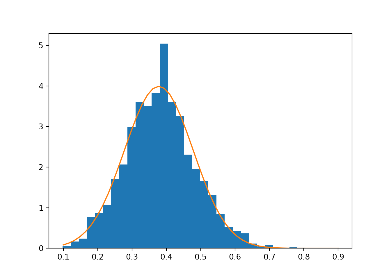
Figure 7.1: Samples from the posterior \(p(\mu | \mathcal{D})\) compared with the analytically derived posterior
7.3 Sampling bounded variables
Many probabilistic models contain variables that have some constraints: variances need to be positive and point probabilities need to be in the interval \([0,1]\).
More formally, let us assume we have a set of variables \(\theta_I\) with bounds \(\theta_I \in B\). There are three possible approaches for dealing with such variables.
7.3.1 Zero likelihood approach
The MH algorithm will converge to the correct distribution under the usual conditions, if the target probability \(P^*(\theta) = 0\) when \(\theta_I \not\in B\). Clearly all moves to such states will be rejected, because the acceptance probability \(a = 0\).
This approach can be quite inefficient, as the sampler will need to propose many moves that are known to be rejected. Considering as an example a symmetric proposal for \(d\) positive variables, starting near the origin. A proposed move that would make even one of the variables negative will be rejected, and hence the probability of acceptance (each variable should be positive) will be of the order \(2^{-d}\).
This approach also requires careful implementation to avoid errors when evaluating densities with a negative variance, for example.
7.3.2 Proposal that respects the bounds
The proposal can be modified to not propose moves that would go outside the bounds.
Example 7.2 Let us consider a sampler for \(\theta_i > 0\). One way to enforce the constraint is to propose \(\theta' = |\theta_0'|\), where \(\theta_0'\) follows some proposal \(q_0(\theta_0' ; \theta)\). This change needs to be taken into account in the evaluation of the proposal density, which will be \[ q(\theta' ; \theta) = \begin{cases} q_0(\theta' ; \theta) + q_0(-\theta' ; \theta), \quad &\theta' > 0, \\ q_0(\theta' ; \theta), & \theta' = 0. \end{cases}\]
Assuming \(q_0(\theta' ; \theta)\) is symmetric with \(q_0(\theta' ; \theta) = q_s(\theta' - \theta)\), with a symmetric \(q_s\), we have \[ q(\theta' ; \theta) = q_s(\theta' - \theta) + q_s(\theta' + \theta),\] which is symmetric and \(q(\theta' ; \theta) = q(\theta ; \theta')\).Such proposals need to be specifically tailored to the problem, which may be complicated if the bounds are complicated. As an example, it is not easy to design a proposal to directly propose symmetric positive-definite matrices.
This kind of special proposals need to be checked whether they are symmetric (\(q(\theta' ; \theta) = q(\theta ; \theta')\)) or if the factor \(\frac{q(\theta^{(t)} ; \theta')}{q(\theta' ; \theta^{(t)})}\) needs to be included in the acceptance ratio.
7.3.3 Transformation to unbounded variables
Samplers for bounded variables can also be implemented using a change of variables through a transformation to unbounded variables.
Let \(\theta_I = g(\phi_I)\), where \(g\) is a smooth invertible transformation such that \(\phi_I \in \mathbb{R}^d\) without any bounds. Typical examples:
- If \(\theta_i > 0\), choose \(g(\phi) = \exp(\phi)\).
- If \(\theta_i \in (0, 1)\), choose \(g(\phi) = 1 / (1 + \exp(-\phi))\), which is known as the logistic transformation.
- If \(\theta_i \in (0, 1), i \in I\) with \(\sum_{i \in I} \theta_i = 1\), \(g_i(\phi) = \frac{\exp(\phi_i)}{\sum_{i' \in I} \exp(\phi_{i'})},\) which is known as the softmax transformation. It should be noted that here \(d\)-dimensional \(\theta_I\) only has \(d-1\) degrees of freedom because of the normalisation requirement.
Transformations of variables need to be taken into account in the probability model.
The likelihood of the model is invariant with respect to transformations of the model parameters, i.e. \[ p(\mathcal{D} | \theta) = p(\mathcal{D} | g(\phi)) = p(\mathcal{D} | \phi), \] but the prior needs to be transformed according to the rule of transformation of probability distributions: \[ p_{\phi}(\phi) = p_{\theta}(g(\phi)) \left| J_g \right|, \] where we have used the rule of transformations of probability densities.
Example 7.3 In the case of transformation for \(\theta_i > 0\) using \(g(\phi) = \exp(\phi)\), we have \[ p(\phi) = p_{\theta}(\exp(\phi)) \exp(\phi). \]
Assuming \(\theta \sim \mathrm{Exponential}(\lambda)\) with \(p(\theta | \lambda) = \lambda \exp(-\lambda \theta)\), we have for \(\phi = \log(\theta):\) \[ p(\phi | \lambda) = \lambda \exp(-\lambda \exp(\phi)) \exp(\phi). \]7.3.4 Sampling with logistic transformed variables
As an example, let us consider sampling over the parameter \(\theta = p \in [0, 1]\) of a binomial model.
We can transform \(\phi \in \mathbb{R}\) to the bounded \(\theta\) using the logistic transformation \[ \mathrm{logistic}(\phi) = \frac{1}{1 + \exp(-\phi)}. \] The inverse transformation from \(\theta\) to \(\phi\) is \[ \mathrm{logistic}^{-1}(\theta) = \log \left(\frac{\theta}{1 - \theta}\right). \]
In order to transform a prior defined for \(\theta\) to one over \(\phi\) for sampling, we will use the transformation \[ p_\phi(\phi) = p_\theta(\mathrm{logistic}(\phi)) \frac{\mathrm{d}}{\mathrm{d}\phi} \mathrm{logistic}(\phi). \] The required derivative of the logistic function can be obtained as \[ \frac{\mathrm{d}}{\mathrm{d}\phi} \mathrm{logistic}(\phi) = \frac{\exp(-\phi)}{\left( 1 + \exp(-\phi)\right)^2}. \]
Let us first define and plot these functions.
def logistic(x):
    return 1/(1+np.exp(-x))

def dlogistic(x):
    return np.exp(-x)/(1+np.exp(-x))**2

def invlogistic(y):
    return np.log(y / (1-y))

fig, ax = plt.subplots(1, 2)
t = np.linspace(-5, 5, 100)
ax[0].plot(t, logistic(t), label="logistic(phi)")
ax[0].plot(t, dlogistic(t), label="logistic'(phi)")
ax[0].legend()
t2 = np.linspace(1e-5, 1-1e-5, 1000)
ax[1].plot(t2, invlogistic(t2))
plt.show()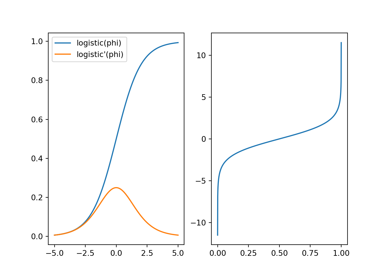
Figure 7.2: Logistic and inverse logistic functions.
We will now apply this transformation for MCMC sampling in a model where \[ p(\mathcal{D} | \theta) = \mathrm{Binom}(k;\; n, \theta) \propto \theta^k (1-\theta)^{n-k}. \] We will use a uniform prior \[ p(\theta) = \mathrm{Uniform}(\theta;\; 0.25, 0.75). \]
# phi in R
# theta = logistic(phi)
# phi = invlogistic(theta)

# un-normalised log-likelihood over theta
def llikelihood(theta, k, n):
    return k*np.log(theta) + (n-k)*np.log(1-theta)

# log-prior over theta
def lprior(theta, lower, upper):
    if theta > lower and theta < upper:
        return np.log(1/(upper-lower))
    else:
        return -np.inf

# transformed log-prior over phi
def lprior_t(phi):
    return lprior(logistic(phi), 0.25, 0.75) + np.log(dlogistic(phi))

# Observations: 60 successes over 100 attempts
k = 60
n = 100

# log-target over phi
def ltarget_t(phi):
    return llikelihood(logistic(phi), k, n) + lprior_t(phi)

# initial value (in theta, needs to be transformed)
theta0 = 0.5
# run the sampler (in phi), notice the proposal in phi space
phi = mhsample1(invlogistic(theta0), 10000,
                ltarget_t, lambda phi: phi + npr.randn(1))
## Sampler acceptance rate: 0.2446## [0.5008244 0.59693608 0.69212267]## (array([0.08976495, 0.58988392, 1.67347505, 4.6806007 , 7.03372462,
## 8.11731574, 6.16813408, 2.55830093, 0.96817905, 0.17952989]), array([0.43425566, 0.46544824, 0.49664082, 0.52783339, 0.55902597,
## 0.59021855, 0.62141113, 0.6526037 , 0.68379628, 0.71498886,
## 0.74618144]), <a list of 10 Patch objects>)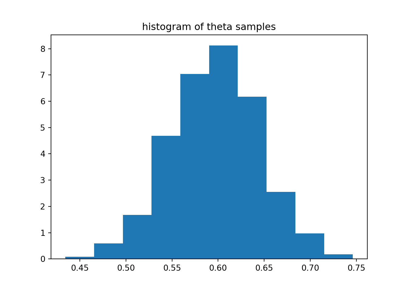
Figure 7.3: Samples from the MCMC example.
7.3.5 Justification for the transformation of densities
The rule for the transformation of densities follows directly from the rule of change of variables for an integral.
Let \(\theta = g(\phi)\), where \(g\) is differentiable with an integrable derivative.
To compute a definite integral of a continuous function \(f(\theta)\), we can use \[ \int\limits_{g(a)}^{g(b)} f(\theta) \,\mathrm{d}\theta = \int\limits_{a}^{b} f(g(\phi)) \frac{\,\mathrm{d} \theta}{\,\mathrm{d} \phi} \,\mathrm{d} \phi. \] This justifies the general change of variables formula \[ f_\phi(\phi) = f_\theta(g(\phi)) \frac{\,\mathrm{d} \theta}{\,\mathrm{d} \phi} = f_\theta(g(\phi)) g'(\phi). \]
Because probability densities need to be positive while \(g'(\phi)\) might not, for probability densities we need to add absolute values to obtain \[ f_\phi(\phi) = f_\theta(g(\phi)) \frac{\,\mathrm{d} \theta}{\,\mathrm{d} \phi} = f_\theta(g(\phi)) |g'(\phi)|. \]
7.3.6 Numerical example of density transformation
Returning to Example 7.3, we can easily numerically verify that these are both valid probability densities:
import scipy.integrate as si
import numpy as np

def p_theta(theta, l):
    return l * np.exp(-l * theta)

def p_phi(phi, l):
    return l * np.exp(-l * np.exp(phi)) * np.exp(phi)

# Note the different bounds for the integrals!
print('p_theta normaliser:', si.quad(lambda theta: p_theta(theta, 2.0), 0, np.inf))
## p_theta normaliser: (0.9999999999999999, 1.547006406148436e-10)print('p_phi normaliser: ', si.quad(lambda phi: p_phi(phi, 2.0), -100, 100))
# Note: setting bounds to infinity would give an error, but
# this range is sufficient in practice## p_phi normaliser: (0.9999999999999987, 2.5196432985839586e-10)We can further see that they yield the same probabilities for events, using \(\theta \in [1, \exp(1)] \Leftrightarrow \phi \in [0, 1]\) as an example here:
# Note the different bounds for the integrals!
print('p_theta probability:', si.quad(lambda theta: p_theta(theta, 2.0), 1, np.exp(1)))
## p_theta probability: (0.13098086236189044, 1.4541796917942933e-15)## p_phi probability: (0.13098086236189044, 1.4541796917942933e-15)References
Gelman, Andrew, John Carlin, Hal Stern, David Dunson, Aki Vehtari, and Donald Rubin. 2013. Bayesian Data Analysis. 3rd ed. Boca Raton, FL: Chapman & Hall/CRC.