Chapter 12 Variational inference
MCMC methods approximate the posterior \(p(\mathbf{\theta} | \mathcal{D})\) through samples. This is convenient because it requires no assumptions about the form of the distribution, but the representation can be inefficient especially in high dimensions.
Variational inference provides an alternative approach: fitting an approximation \(q(\mathbf{\theta}) \approx p(\mathbf{\theta} | \mathcal{D})\) with a simple functional form, such as a suitable normal distribution, and casting the inference task as an optimisation problem. Because of its suitability to high-dimensional problems, variational inference is popular especially in machine learning. As a rule of thumb, variational inference is typically at least 10x faster than comparable MCMC.
Variational algorithms can often find good approximations of posterior means, but often underestimate the posterior variances. This is illustrated in Fig. 12.1, which compares posterior distributions over inferred gene transcript expression levels from MCMC and variational inference (denoted VB) for a large number of transcripts. The figure shows that the mean estimates of the two methods are essentially identical while variational inference often underestimates the variance.
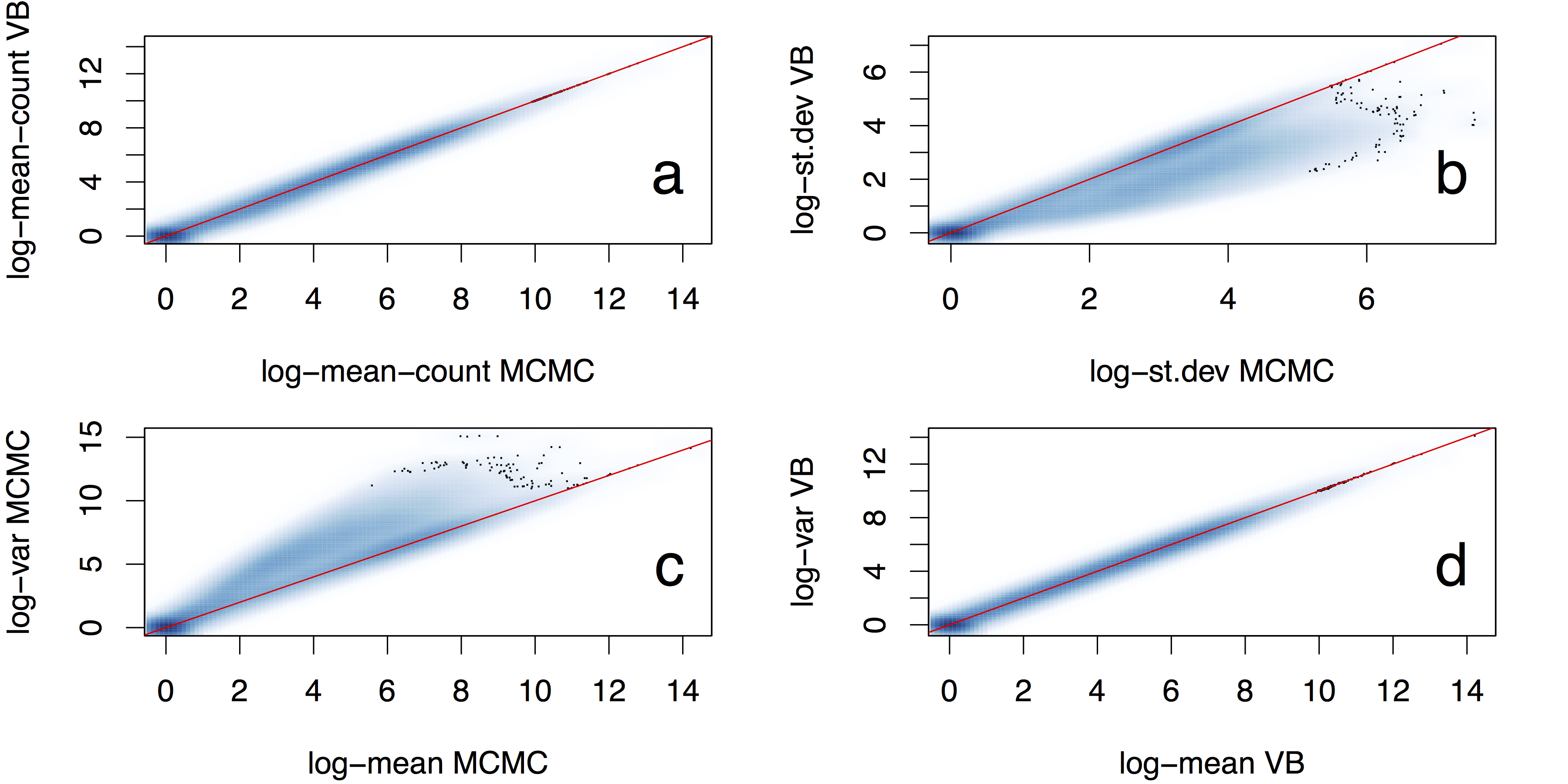
Figure 12.1: Comparison of posterior means and standard deviations over gene transcript expression levels inferred using MCMC and variational inference (denoted VB) (Hensman et al., Fast and accurate approximate inference of transcript expression from RNA-seq data. Bioinformatics 2015).
12.1 Variational inference basics
Variational inference (VI) is based on fitting an approximation \(q(\theta)\) to the posterior by minimising the Kullback–Leibler divergence \[ D_{KL}(q(\theta) || p(\theta | \mathcal{D})) = \mathrm{E}_{q(\theta)}\left[\log \frac{q(\theta)}{p(\theta | \mathcal{D})} \right] \] between the approximation and the true posterior.
Kullback–Leibler divergence has some properties of a distance, but it is asymmetric and hence not a proper metric. Nevertheless it satisfies: \[\begin{align*} D_{KL}(q || p) &\ge 0 \quad \forall q, p \\ D_{KL}(q || p) &= 0 \quad \Leftrightarrow \quad q = p \; \text{(a.e.)}. \end{align*}\]
Exact Kullback–Leibler divergence usually difficult to compute, so the so-called evidence lower-bound (ELBO) is used instead: \[ \mathcal{L} = \mathrm{E}_{q(\theta)}\left[\log \frac{p(\theta, \mathcal{D})}{q(\theta)} \right] = \log p(\mathcal{D}) - D_{KL}(q(\theta) || p(\theta | \mathcal{D})). \] Because \[ D_{KL}(q(\theta) || p(\theta | \mathcal{D})) \ge 0, \] we have \[ \mathcal{L} \le \log p(\mathcal{D}). \] The name ELBO comes from the alternative name evidence of the marginal likelihood \(p(\mathcal{D})\).
Optimising the ELBO serves a dual purpose: the minimiser \(q(\theta)\) yields the best approximation of the posterior \(p(\theta | \mathcal{D})\) in terms of the Kullback–Leibler divergence, and the value provides an approximation (bound) on the marginal likelihood, which can be used for model comparison.
12.2 Classical variational inference
Classical algorithms for VI, also known as variational EM algorithms, are based on cyclic optimisation of \(\mathcal{L}\) one variable at a time while keeping others fixed, similar to Gibbs sampling.
This can usually be performed for the same kind of models where Gibbs sampling can be applied: models where the conditional posterior of a single variable given others can be expressed in closed form.
Derivation of the updates can be quite tedious because of the expectations over \(q(\theta)\) that are required.
12.3 Doubly stochastic variational inference (DSVI) and Automatic differentiation variational inference (ADVI)
DSVI and ADVI are based on the idea of simplifying the derivation by Monte Carlo evaluation of expectations over \(q(\theta)\).
The algorithms make extensive use of the reparametrisation trick: gradients of the expectations \[ E_{q(\mathbf{\theta})}[ \cdot ] \] with respect to a changing distribution such as \[ q(\mathbf{\theta}) = \mathcal{N}(\mathbf{\theta};\; \mathbf{\mu}, \mathbf{\Sigma}) \] can be turned to expectations with respect to a fixed distribution via reparametrisation \[ \mathbf{\theta} = \mathbf{L} \mathbf{\eta} + \mathbf{\mu}, \] where \(\mathbf{\eta} \sim \mathcal{N}(\mathbf{0}, \mathbf{I})\) and \(\mathbf{L}\) is the Cholesky factor of \(\mathbf{\Sigma}\) satisfying \(\mathbf{L} \mathbf{L}^T = \mathbf{\Sigma}\).
The ELBO can now be written as \[\begin{align*} \mathcal{L} &= \mathrm{E}_{q(\boldsymbol{\theta})}\left[\log \frac{p(\boldsymbol{\theta}, \mathcal{D})}{q(\boldsymbol{\theta})} \right] \\ &= \int q(\boldsymbol{\theta}) \log \frac{p(\boldsymbol{\theta}, \mathcal{D})}{q(\boldsymbol{\theta})} \mathrm{d}\boldsymbol{\theta} \\ &= \int \phi(\boldsymbol{\eta}) \log \frac{p(\mathbf{L} \boldsymbol{\eta} + \boldsymbol{\mu}, \mathcal{D}) |\mathbf{L}|}{\phi(\boldsymbol{\eta})} \mathrm{d}\boldsymbol{\eta}, \end{align*}\] where \(\phi(\boldsymbol{\eta})\) is the density of \(\boldsymbol{\eta}\) and \(|\mathbf{L}|\) comes from the coordinate transformation. We can thus write \[ \mathcal{L} = \mathrm{E}_{\phi(\mathbf{\eta})}[\log p(\mathbf{L} \mathbf{\eta} + \mathbf{\mu}, \mathcal{D})] + \log |\mathbf{L}| + \mathrm{E}_{\phi(\mathbf{\eta})}[ -\log \phi(\mathbf{\eta})]. \] As \(\mathbf{L}\) is a triangular matrix, its determinant \(|\mathbf{L}| = \prod_{i=1}^{d} l_{ii}\) and thus \(\log |\mathbf{L}| = \sum_{i=1}^{d} \log l_{ii}\).
The gradients with respect to \(\mu\) and \(\mathbf{L}\) can be obtained by ignoring the last constant term and changing the order of derivation and integration as \[\begin{align*} \nabla_{\boldsymbol{\mu}} \mathcal{L} &= \mathrm{E}_{\phi(\boldsymbol{\eta})}[\nabla_{\boldsymbol{\mu}} \log p(\mathbf{L} \boldsymbol{\eta} + \boldsymbol{\mu}, \mathcal{D})] \\ &= \mathrm{E}_{\phi(\boldsymbol{\eta})}[\nabla_{\boldsymbol{\theta}} \log p(\boldsymbol{\theta}, \mathcal{D})] \\ \nabla_{\mathbf{L}} \mathcal{L} &= \mathrm{E}_{\phi(\boldsymbol{\eta})}[\nabla_{\mathbf{L}} \log p(\mathbf{L} \boldsymbol{\eta} + \boldsymbol{\mu}, \mathcal{D})] + \Delta_{\mathbf{L}} \\ &= \mathrm{E}_{\phi(\boldsymbol{\eta})}[\nabla_{\boldsymbol{\theta}} \log p(\boldsymbol{\theta}, \mathcal{D})] \times \boldsymbol{\eta}^T + \Delta_{\mathbf{L}}, \end{align*}\] where \(\Delta_{\mathbf{L}} = \mathrm{diag}(1/l_{11}, \dots, 1/l_{dd})\).
The required expectations with respect to \(\phi(\mathbf{\eta})\) can be evaluated using Monte Carlo. In many cases using just 1 Monte Carlo sample will provide sufficient accuracy for stochastic gradient optimisation. The gradients required can usually be easily evaluated using automatic differentiation, making the implementation of the method straightforward.
In order to decrease the amount of computation, it is also possible to restrict \(\mathbf{\Sigma}\) to be a diagonal matrix. In this case \(\mathbf{L}\) will also be diagonal with \(l_{ii}^2\) corresponding to the approximate posterior variance of \(\theta_i\) in \(q(\theta_i)\).
12.4 Stochastic optimisation for variational inference
Using Monte Carlo for expectations \(\mathrm{E}_{\phi(\mathbf{\eta})}[\cdot]\) we can obtain approximate gradients \(\tilde{\nabla}_{\mathbf{\mu}} \mathcal{L}\), \(\tilde{\nabla}_{\mathbf{L}} \mathcal{L}\).
We can maximise \(\mathcal{L}\) with stochastic gradient ascent \[\begin{align*} \boldsymbol{\mu}_{t+1} &= \boldsymbol{\mu}_t + \rho_t \tilde{\nabla}_{\boldsymbol{\mu}} \mathcal{L}(\boldsymbol{\mu}_t, \mathbf{L}_t) \\ \mathbf{L}_{t+1} &= \mathbf{L}_t + \rho_t \tilde{\nabla}_{\mathbf{L}} \mathcal{L}(\boldsymbol{\mu}_t, \mathbf{L}_t) \end{align*}\] where the step sizes \(\rho_t\) need to satisfy \[\begin{align*} \sum_{t=1}^\infty \rho_t &= \infty \\ \sum_{t=1}^\infty \rho_t^2 &< \infty \end{align*}\] to guarantee convergence.
12.5 Example
We will now redo Example 7.1 with variational inference. In the example, the target joint distribution is \[ \log p(\mathcal{D}, \mu) = \log p(\mathcal{D} | \mu) + \log p(\mu) = \sum_{i=1}^n \log \mathcal{N}(x_i ;\; \mu, \sigma_x^2) + \log \mathcal{N}(\mu ;\; \mu_0, \sigma_0^2). \]
We again use the parameters at \(\sigma_x^2 = 1, \mu_0 = 0, \sigma_0^2 = 3^2\).
We use the normal approximation \[ q(\mu) = \mathcal{N}(\mu';\; \bar{\mu}, \tilde{\mu}^2), \] which can be reparametrised using \[ \mu = \bar{\mu} + \tilde{\mu} \eta_\mu, \] where \(\eta_\mu \sim \mathcal{N}(0, 1)\). The stochastic gradient algorithm for fitting the variational approximation can be implemented as follows. The resulting approximation and the corresponding analytical posterior are compared in Fig. 12.3.
12.5.1 Autograd
import autograd.numpy as np
import autograd
import matplotlib.pyplot as plt

# Define the normal pdf. Note parameters: mean, standard deviation
def lnormpdf(x, mu, sigma):
    return -0.5*np.log(2*np.pi) - np.log(sigma) - 0.5 * (x-mu)**2/sigma**2

# Doubly stochastic variational inference
# Algorithm 1 of Titsias and Lázaro-Gredilla (2014)
def dsvi(m0, c0, gradient, sample_eta, rho0, t0 = 100, niters = 10000):
    """Doubly stochastic variational inference from
    Algorithm 1 of Titsias and Lázaro-Gredilla (2014)
    Arguments:
    m0: initial value of mean (scalar)
    c0: initial value of standard deviation (scalar)
    logjoint: function returning the value of the log-joint distribution p(X, theta)
    sample_eta: function sampling fixed parameters eta
    rho0: initial learning rate the rho_t = rho0 / (t0 + t)
    t0: t0 for the above (default: 100)
    niters: number of iterations (default: 10000)"""
    m = m0
    c = c0
    mhist = np.zeros(niters)
    chist = np.zeros(niters)
    for t in range(niters):
        eta = sample_eta()
        theta = c * eta + m
        g = gradient(theta)
        m = m + rho0 / (t0 + t) * g
        c = c + rho0 / (t0 + t) * (g * eta + 1/c)
        mhist[t] = m
        chist[t] = c
    return m, c, mhist, chist

# Simulate n=100 points of normally distributed data about mu=0.5
n = 100
data = 0.5 + npr.normal(size=n)

# Set the prior parameters
sigma_x = 1.0
mu0 = 0.0
sigma0 = 3.0

# Define the target log-pdf as a sum of likelihood and prior terms
def logjoint(mu, data=data, sigma_x=sigma_x, mu0=mu0, sigma0=sigma0):
    return lnormpdf(data, mu, sigma_x).sum() + lnormpdf(mu, mu0, sigma0)

m, c, mhist, chist = dsvi(1.0, 1.0, autograd.grad(logjoint), npr.normal, 0.1)
print(m, c)
## 0.46316880777800606 0.09957996518556934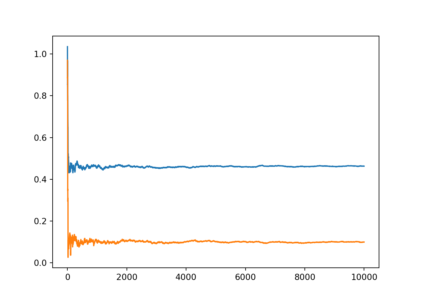
Figure 12.2: Convergence of the parameters of the variational approximation during stochastic optimisation with Autograd.
tt = np.linspace(0.1, 0.9, 50)
m_post = sigma0**2 * np.sum(data) / (n*sigma0**2 + sigma_x**2)
s2_post = 1/(n/sigma_x**2 + 1/sigma0**2)
y = np.exp(lnormpdf(tt, m_post, np.sqrt(s2_post)))
plt.plot(tt, y, label='exact')
# Note: c is +/- sqrt(variance), need abs() to get standard deviation!
y_vi = np.exp(lnormpdf(tt, m, np.abs(c)))
plt.plot(tt, y_vi, label='variational approximation')
plt.legend()
plt.show()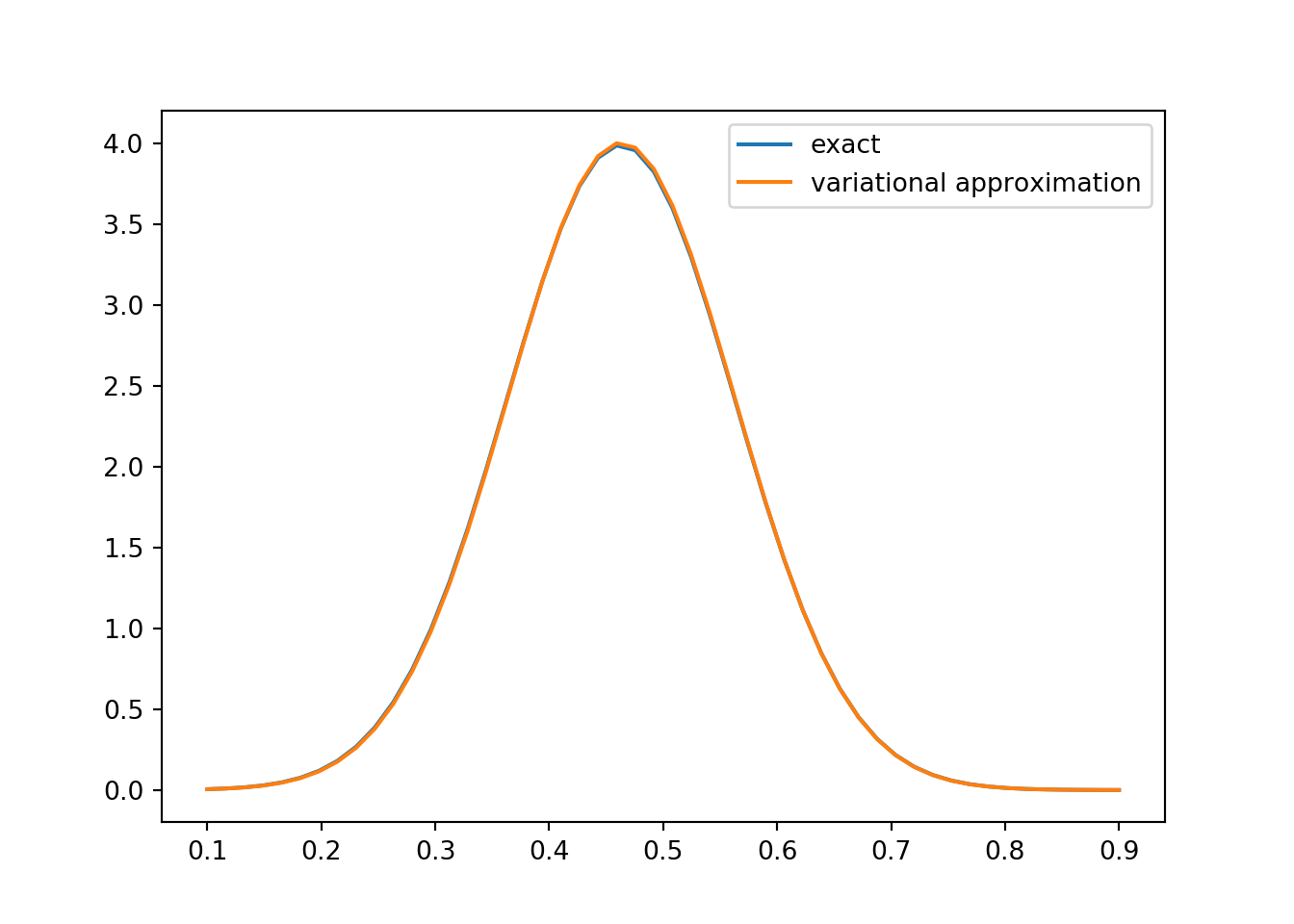
Figure 12.3: Variational approximation to the posterior \(p(\mu | \mathcal{D})\) compared with the analytically derived posterior
12.5.2 PyTorch
import torch
import math
import matplotlib.pyplot as plt

torch.set_default_dtype(torch.double)
# Uncomment this to run on GPU
# torch.set_default_tensor_type(torch.cuda.DoubleTensor)

# Define the normal pdf. Note parameters: mean, standard deviation
def lnormpdf(x, mu, sigma):
    return (-0.5*math.log(2*math.pi)
            -torch.log(torch.tensor(sigma)) -0.5*(x-mu)**2/sigma**2)

def dsvi(m0, c0, logjoint, sample_eta, rho0, t0 = 100, niters = 10000):
    """Doubly stochastic variational inference from
    Algorithm 1 of Titsias and Lázaro-Gredilla (2014)
    Arguments:
    m0: initial value of mean (tensor of length 1)
    c0: initial value of standard deviation (tensor of length 1)
    logjoint: function returning the value of the log-joint distribution p(X, theta)
    sample_eta: function sampling fixed parameters eta
    rho0: initial learning rate the rho_t = rho0 / (t0 + t)
    t0: t0 for the above (default: 100)
    niters: number of iterations (default: 10000)"""
    m = m0
    c = c0
    mhist = torch.zeros(niters)
    chist = torch.zeros(niters)
    for t in range(niters):
        eta = sample_eta()
        theta = (c * eta + m).detach().requires_grad_(True)
        v = logjoint(theta)
        v.backward()
        g = theta.grad
        m = m + rho0 / (t0 + t) * g
        c = c + rho0 / (t0 + t) * (g * eta + 1/c)
        theta.grad.zero_()
        mhist[t] = m
        chist[t] = c
    return m, c, mhist, chist

# Set the seed for PyTorch RNGs
torch.manual_seed(42)
# Simulate n=100 points of normally distributed data about mu=0.5
## <torch._C.Generator object at 0x7fa887999af0>n = 100
data = 0.5 + torch.randn(n)
# Set the prior parameters
sigma_x = 1.0
mu0 = 0.0
sigma0 = 3.0
# Define the target log-pdf as a sum of likelihood and prior terms
def logjoint(mu, data=data, sigma_x=sigma_x, mu0=mu0, sigma0=sigma0):
return lnormpdf(data, mu, sigma_x).sum() + lnormpdf(mu, mu0, sigma0)
m, c, mhist, chist = dsvi(1.0, 1.0, logjoint, lambda: torch.randn(1), 0.1)
print(m.item(), c.item())## 0.6605256723408588 0.09835959585228018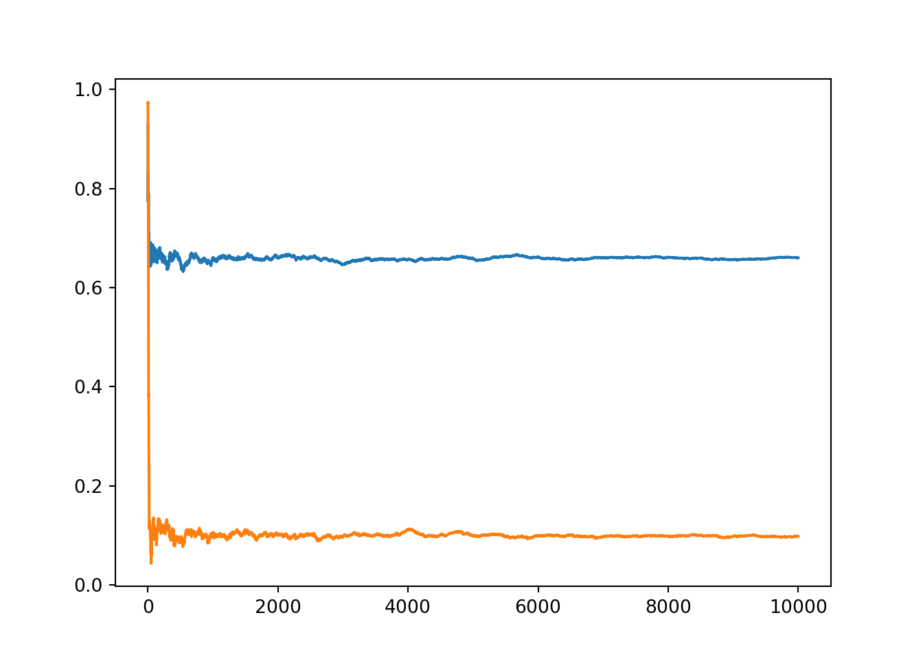
Figure 12.4: Convergence of the parameters of the variational approximation during stochastic optimisation with PyTorch.
12.6 Final notes
Variational methods provide an approach to approximate inference by casting the method as an optimisation problem. The result is an approximation: unlike MCMC it will not converge to the exact posterior no matter how long the algorithm is run.
Classical methods of variational inference only apply to quite restricted set of models and can require tedious derivations to implement.
References
Kucukelbir, Alp, Dustin Tran, Rajesh Ranganath, Andrew Gelman, and David M. Blei. 2017. “Automatic Differentiation Variational Inference.” Journal of Machine Learning Research 18: 14:1–14:45. http://jmlr.org/papers/v18/16-107.html.
Titsias, Michalis K., and Miguel Lázaro-Gredilla. 2014. “Doubly Stochastic Variational Bayes for Non-Conjugate Inference.” In Proceedings of the 31th International Conference on Machine Learning, ICML 2014, Beijing, China, 21-26 June 2014, 1971–9. http://proceedings.mlr.press/v32/titsias14.html.