Chapter 5 Density estimation and cross validation
Many statistical concepts rely on smooth probability densities. If we are only given a finite sample, it will only cover a discrete set of points and as such provides no clues on the probability of other points or the density.
Parametric models provide a common approach for obtaining a smooth probability model over some data. For example, given a sample \(X\), we can fit a probability model \(p(x)\) if we assume that \(X\) follow the normal distribution and match the mean and variance of \(p(x)\) with the sample mean and variance of \(X\). This model provides a smooth probability density, but makes the big assumption that the data follow a normal distribution, which is a very restrictive assumption.
In this chapter we study kernel density estimation, which provides a means of obtaining a smooth probability density from a sample of points without assuming a specific functional form for the density. One of the key challenges in applying kernel density estimation is how to determine the smoothness of the density. We use this problem to illustrate cross validation, which is a very useful general method for estimating unknown parameters.
5.1 Kernel density estimation
The basic idea of kernel density estimation is to place a small bump called a kernel \(K_h(x)\) around every observation. Averaging these bumps together yields the desired probability density.
Formally, given a sample \(X = (x_1, x_2, \dots, x_n)\) and a kernel \(K(x)\) that satisfies \[ \int_{-\infty}^{\infty} K(x) \mathrm{d}x = 1, \] the kernel density estimate \(f_h(t)\) is \[ f_h(t) = \frac{1}{nh} \sum_{i=1}^n K\left(\frac{t - x_i}{h}\right), \] where \(h\) denotes the width of the kernel, often called kernel bandwidth.
Common choices of the kernel include the Gaussian kernel that follows the standard normal probability density function \[ K_{\text{gauss}}(x) = \frac{1}{\sqrt(2 \pi)} \exp\left(\frac{-x^2}{2}\right), \] the uniform kernel \[ K_{\text{uniform}}(x) = \begin{cases}\frac{1}{2} \quad & \text{if } |x|<1, \\ 0 & \text{otherwise},\end{cases} \] and the Epanechnikov kernel \[ K_{\text{Epanechnikov}}(x) = \begin{cases}\frac{3}{4}(1 - x^2) \quad & \text{if } |x|<1, \\ 0 & \text{otherwise}.\end{cases} \]
These kernels are illustrated below in Fig. 5.1.
import numpy as np
import pandas as pd
import matplotlib.pyplot as plt

def K_gauss(x):
    return np.exp(-x**2/2) / np.sqrt(2*np.pi)

def K_uniform(x):
    return 0.5*(np.abs(x) < 1)

def K_epanechnikov(x):
    return 3/4*(1-x**2)*(np.abs(x) < 1)

t = np.linspace(-3, 3, 100)
plt.plot(t, K_gauss(t), label='K_Gauss')
plt.plot(t, K_uniform(t), label='K_uniform')
plt.plot(t, K_epanechnikov(t), label='K_Epanechnikov')
plt.legend()
plt.show()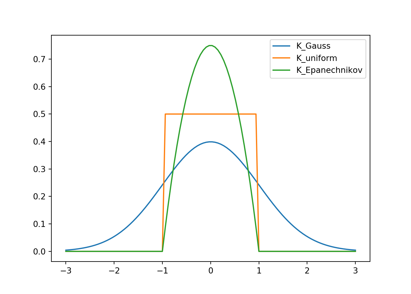
Figure 5.1: Illustration of 1D kernels.
The specific choice of the kernel is usually not that important. The Gaussian kernel has the benefit of being smooth, which implies that the resulting \(f_h(t)\) will be smooth as well. On the other hand, the Gaussian kernel is non-zero over the entire real line, which means that every term in the sum for \(f_h(t)\) will be non-zero. It may be computationally more advantageous to use one of the other kernels that are non-zero only on a finite interval, thus making the sum sparse.
An example to illustrate kernel density estimation with the Gaussian
kernel is provided in Fig. 5.2, the code for which is
given below. The kernel_density() code is made more complicated
because it accepts both a scalar value and a numpy.array as input.
import numpy as np
import pandas as pd
import matplotlib.pyplot as plt

d = pd.read_csv('http://www.cs.helsinki.fi/u/ahonkela/teaching/compstats1/toydata.txt').values

plt.hist(d, 30, density=True)
## (array([0.0064341 , 0.0064341 , 0.        , 0.0128682 , 0.04503872,
##        0.11581384, 0.10294564, 0.21232538, 0.24449589, 0.21232538,
##        0.31527102, 0.25093   , 0.2573641 , 0.23806179, 0.19945718,
##        0.19945718, 0.14798436, 0.14798436, 0.16728666, 0.10937974,
##        0.09651154, 0.03217051, 0.04503872, 0.01930231, 0.0128682 ,
##        0.0064341 , 0.        , 0.        , 0.        , 0.0064341 ]), array([8.7330000e-03, 3.2019960e-01, 6.3166620e-01, 9.4313280e-01,
##        1.2545994e+00, 1.5660660e+00, 1.8775326e+00, 2.1889992e+00,
##        2.5004658e+00, 2.8119324e+00, 3.1233990e+00, 3.4348656e+00,
##        3.7463322e+00, 4.0577988e+00, 4.3692654e+00, 4.6807320e+00,
##        4.9921986e+00, 5.3036652e+00, 5.6151318e+00, 5.9265984e+00,
##        6.2380650e+00, 6.5495316e+00, 6.8609982e+00, 7.1724648e+00,
##        7.4839314e+00, 7.7953980e+00, 8.1068646e+00, 8.4183312e+00,
##        8.7297978e+00, 9.0412644e+00, 9.3527310e+00]), <a list of 30 Patch objects>)
def K_gauss(x):
return 1/np.sqrt(2*np.pi)*np.exp(-0.5*x**2)
def kernel_density(t, x, h):
"""Return kernel density at t estimated for points x with width h
Input: t (np.array, shape (k, )) for k points or float for 1 point
x (np.array, shape (n, )) for n points
h double"""
try:
N = len(t)
except: # t is a scalar value if it has no length
t = np.array([t])
N = 1
y = np.zeros(N)
for i in range(N):
y[i] = np.mean(K_gauss((t[i] - x)/ h)) / h
return y
t = np.linspace(-2, 10, 100)
plt.plot(t, kernel_density(t, d, 3.0), label='h=3.0')
plt.plot(t, kernel_density(t, d, 1.0), label='h=1.0')
plt.plot(t, kernel_density(t, d, 0.3), label='h=0.3')
plt.plot(t, kernel_density(t, d, 0.1), label='h=0.1')
plt.legend()
plt.show()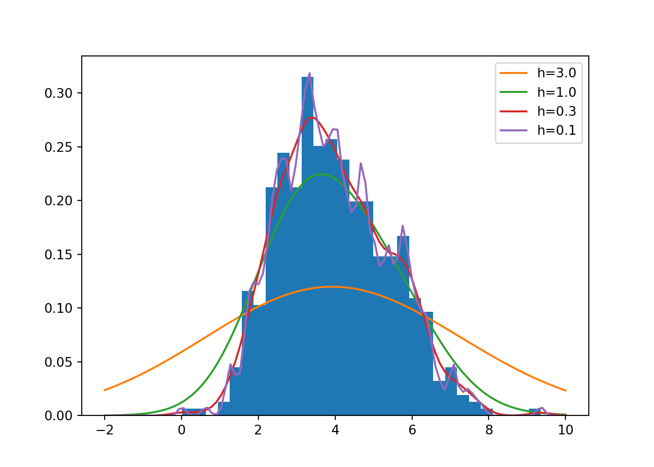
Figure 5.2: Illustration of kernel density estimation with the Gaussian kernel.
5.1.1 Multivariate density estimation
The above discussion can be generalised to the \(d\)-dimensional case by writing the kernel density estimate \(f_h(x)\) as \[ f_h(\mathbf{x}) = \frac{1}{nh^d} \sum_{i=1}^n K\left(\frac{\mathbf{x} - \mathbf{x}_i}{h}\right). \]
The Gaussian and the uniform kernel generalise to the \(d\)-dimensional case easily as \[ K_{\text{gauss}}(\mathbf{x}) = (2 \pi)^{-d/2} \exp\left(\frac{-\|\mathbf{x}\|^2}{2}\right) \] \[ K_{\text{uniform}}(\mathbf{x}) = \begin{cases}\frac{1}{2^d} \quad & \text{if } \|\mathbf{x}\|_{\infty}<1, \\ 0 & \text{otherwise},\end{cases} \] where \(\|\mathbf{x}\|_{\infty} = \max_{i = 1,\dots,d} |x_i|\).
Contour plots of these kernels are illustrated below in Fig. 5.3.
import numpy as np
import pandas as pd
import matplotlib.pyplot as plt

def k_ndgauss(x):
    """Gaussian kernel
    Input: x (np.array, shape (n, d)) for n points with d dimensions"""
    d = x.shape[1]
    return np.exp(-np.sum(x**2, 1)/2) / np.sqrt(2*np.pi)**d

def k_nduniform(x):
    """Uniform kernel
    Input: x (np.array, shape (n, d)) for n points with d dimensions"""
    d = x.shape[1]
    return (0.5)**d * np.all((np.abs(x) < 1), 1)

# Create plotting region
t = np.linspace(-3, 3, 100)
# Create two matrices of X and Y coordinates of points in the region
[X, Y] = np.meshgrid(t, t)
Z_gauss = np.zeros(X.shape)
Z_uniform = np.zeros(X.shape)

# For each column of inputs, evaluate the kernels
# using hstack() with column vectors to create the data matrices
for i in range(X.shape[1]):
    Z_gauss[:,i] = k_ndgauss(np.hstack((X[:, i:i+1], Y[:, i:i+1])))
    Z_uniform[:,i] = k_nduniform(np.hstack((X[:, i:i+1], Y[:, i:i+1])))
fig, ax = plt.subplots(1, 2)
ax[0].contour(X, Y, Z_gauss)
## <matplotlib.contour.QuadContourSet object at 0x7fa8878e7880>## <matplotlib.contour.QuadContourSet object at 0x7fa8878e7850>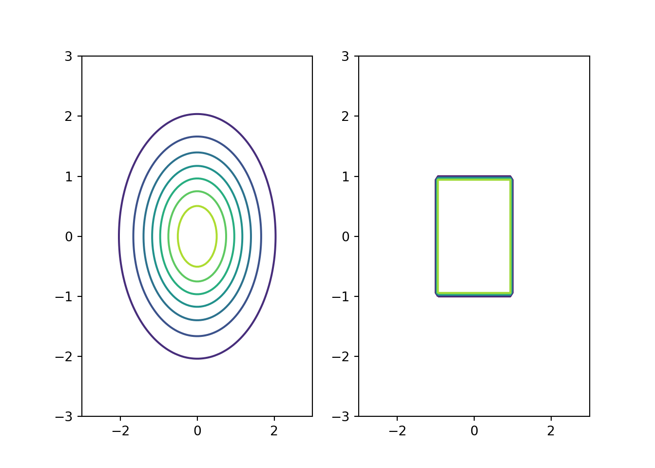
Figure 5.3: Illustration of 2D kernels: Gaussian (left) and uniform (right).
5.2 Cross-validation (CV)
Cross-validation (CV) provides a general, conceptually simple and widely applicable method for estimating unknown parameters from data.
A general CV procedure proceeds as follows:
- Randomly partition the data set \(X = (x_1, x_2, \dots, x_n)\) to a training set \(X_\text{train}\) (\(n-m\) samples) and a test set \(X_\text{test}\) (\(m\) samples)
- Fit the model (estimate density) using \(X_\text{train}\)
- Test the fitted model using \(X_\text{test}\)
- Repeat \(t\) times and average the results
Some example realisations of the CV procedure:
- \(k\)-fold CV: fixed partition to \(k\) equal subsets, \(m=n/k\), \(t=k\) testing on every subset once
- Leave-one-out (LOO) CV: \(m=1\), \(t=n\) testing on every sample once (also \(k\)-fold CV with \(k=n\))
- Monte Carlo CV: randomly sample subsets of suitable size for the desired number of times
5.2.1 CV for kernel bandwidth selection
Let us consider the application of CV and specifically LOO-CV to the problem of selection of the kernel bandwidth \(h\).
Let us denote by \(f_{\setminus i,h}(x)\) the probability density fitted to \(X \setminus \{ x_i \}\).
The LOO objective is \[ LOO(h) = \sum_{i=1}^n \frac{1}{n} \log f_{\setminus i, h}(x_i), \] i.e. we evaluate the mean of the log-probabilities of the test points.
This is illustrated in the example below, where LOO-CV finds a reasonable estimate of \(h\), as seen in Fig. 5.4.
import numpy as np
import pandas as pd
import matplotlib.pyplot as plt

def cross_validate_density(d):
    hs = np.linspace(0.1, 1.0, 10)
    logls = np.zeros(len(hs))
    for j in range(len(d)):
        for i in range(len(hs)):
            logls[i] += np.sum(np.log(kernel_density(d[j], np.delete(d, j), hs[i])))
    return (hs, logls)

hs, logls = cross_validate_density(d)

plt.hist(d, 30, density=True)
## (array([0.0064341 , 0.0064341 , 0. , 0.0128682 , 0.04503872,
## 0.11581384, 0.10294564, 0.21232538, 0.24449589, 0.21232538,
## 0.31527102, 0.25093 , 0.2573641 , 0.23806179, 0.19945718,
## 0.19945718, 0.14798436, 0.14798436, 0.16728666, 0.10937974,
## 0.09651154, 0.03217051, 0.04503872, 0.01930231, 0.0128682 ,
## 0.0064341 , 0. , 0. , 0. , 0.0064341 ]), array([8.7330000e-03, 3.2019960e-01, 6.3166620e-01, 9.4313280e-01,
## 1.2545994e+00, 1.5660660e+00, 1.8775326e+00, 2.1889992e+00,
## 2.5004658e+00, 2.8119324e+00, 3.1233990e+00, 3.4348656e+00,
## 3.7463322e+00, 4.0577988e+00, 4.3692654e+00, 4.6807320e+00,
## 4.9921986e+00, 5.3036652e+00, 5.6151318e+00, 5.9265984e+00,
## 6.2380650e+00, 6.5495316e+00, 6.8609982e+00, 7.1724648e+00,
## 7.4839314e+00, 7.7953980e+00, 8.1068646e+00, 8.4183312e+00,
## 8.7297978e+00, 9.0412644e+00, 9.3527310e+00]), <a list of 30 Patch objects>)## Optimal h: 0.5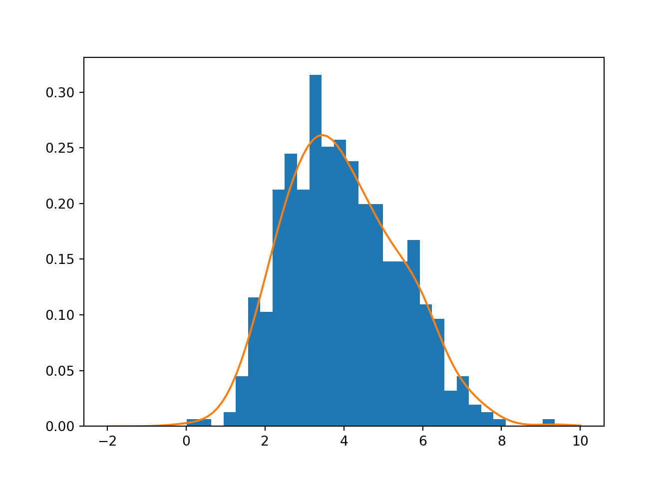
Figure 5.4: Illustration of cross-validation for kernel bandwidth estimation
CV is a widely used too especially in machine learning. Givens and Hoeting (2013) however warn that in the context of kernel bandwidth estimation, the result may be sensitive to high sampling variability and other heuristic methods may be more reliable.
5.3 Other methods for kernel bandwidth selection
The problem of choice of the kernel bandwidth \(h\) is in many cases inherently ill-posed. To analyse the problem, we consider measures that can be used to evaluate the performance of the density estimate \(\hat{f}_h(x)\), when the true density is assumed to be \(f(x)\).
The first measure is the squared \(L_2\) distance, which is in this context often called the integrated squared error (ISE), \[ \mathrm{ISE}(h) = \int_{-\infty}^\infty (\hat{f}_h(x) - f(x))^2 \,\mathrm{d} x. \] \(\mathrm{ISE}(h)\) depends on the observed sample, and to avoid this dependence one can define the mean integrated squared error (MISE) \[ \mathrm{MISE}(h) = \operatorname{E}\left[ \int_{-\infty}^\infty (\hat{f}_h(x) - f(x))^2 \,\mathrm{d} x \right], \] where the expectation is taken with respect to the true density \(f(x)\). By changing the order of expectation and integration, we obtain \[ \mathrm{MISE}(h) = \int_{-\infty}^\infty \operatorname{E}[ (\hat{f}_h(x) - f(x))^2 ] \,\mathrm{d} x, \] which is also known as the integrated mean squared error (IMSE).
By denoting \[ R(g) = \int_{-\infty}^\infty g^2(z) \,\mathrm{d} z \] and assuming \(R(K) < \infty\) and that \(f\) is sufficiently smooth, i.e. \(f\) has two bounded continuous derivatives and \(R(f'') < \infty\), one can derive an expression for \(\mathrm{MISE}(h)\) as (Givens and Hoeting (2013)) \[ \mathrm{MISE}(h) = \frac{R(K)}{nh} + \frac{h^4 \sigma_K^4 R(f'')}{4} + \mathcal{O}\left(\frac{1}{nh}+h^4\right). \] If \(h \rightarrow 0\) and \(nh \rightarrow \infty\) as \(n \rightarrow \infty\), \(\mathrm{MISE}(h) \rightarrow 0\). Minimising the two first terms with respect to \(h\) yields the optimal bandwidth (Givens and Hoeting (2013)) \[ h = \left( \frac{R(K)}{n \sigma_K^4 R(f'')} \right)^{1/5}. \] As the expression depends on the unknown \(R(f'')\), it is not directly useful in selecting \(h\), but it tells the optimal bandwidth \(h\) should decrease as \(h = \mathcal{O}(n^{-1/5})\) in which case the error will decrease as \(\mathrm{MISE} = \mathcal{O}(n^{-4/5})\).
5.4 Literature
Givens and Hoeting (2013) provide an accessible overview of kernel density estimation.
References
Givens, Geof H., and Jennefer A. Hoeting. 2013. Computational Statistics. 2nd ed. Hoboken, NJ: Wiley.